Spatio-Temporal Accessibility of Pharmacy Care in Vermont, USA
Authors
- Sam Roubin, sroubin@middlebury.edu, https://orcid.org/0009-0005-5490-3744, Middlebury College
- Joseph Holler*, josephh@middlebury.edu, https://orcid.org/0000-0002-2381-2699, Middlebury College
- Peter Kedron, peterkedron@ucsb.edu, https://orcid.org/0000-0002-1093-3416, University of California, Santa Barbara
* Corresponding author
Abstract
Pharmacy care is a fundamental aspect of primary healthcare and is gaining greater recognition in the healthcare landscape. Recent research has underscored the importance of pharmacy access in primary care, as pharmacies are visited at higher rates than primary care providers and are valuable for reaching underserved and rural populations. We aim to measure spatiotemporal variation in access to pharmacy care across the state of Vermont using the enhanced 2-step floating catchment area (E2SFCA) method. Specifically, we seek to identify areas that have particularly limited access to pharmacies. This research is temporally explicit, as it analyzes variation in accessibility at specific times of the day and days of the week. Such temporally granular data provides information on how spatial accessibility varies at irregular times, improving our understanding of when pharmacy care is particularly limited for certain populations. Our findings reveal significant disparities in pharmacy access between rural towns and metropolitan and micropolitan towns across virtually all temporal segments. Accessibility was diminished during weekends across all town types, highlighting potential challenges in accessing care outside of conventional business hours. Accessibility gaps between rural and urban areas were exacerbated outside of standard weekday business hours. Few studies have used the two-step floating catchment area (2SFCA) and the E2SFCA method to measure spatial accessibility of pharmacy care across geographic scales and regions. To our knowledge, this is the first temporally explicit study of pharmacy care and the first E2SFCA study of pharmacy accessibility in Vermont. Our results may be of interest to service providers and Vermont state public health officials with important implications for public health planning in the state.
This study adapts and extends the methodology used in Kang et al.'s (2020) "Rapidly measuring spatial accessibility of COVID-19 healthcare resources: a case study of Illinois, USA" to measure spatial accessibility of pharmacy care across Vermont.
Study metadata
Key words
: Pharmacy, spatial accessibility, pharmacy deserts, Vermont, E2FSCA.Subjects
:- Medicine and Health Sciences: Public Health: Health Services Research
- Social and Behavioral Sciences: Geography: Geographic Information Sciences
- Social and Behavioral Sciences: Geography: Human Geography
Date created
: 18-Sept-2023Date modified
: 6-Sept-2024Spatial Coverage
: The state of Vermont and areas within 10-miles of the Vermont border (MA, NY, NH). Canada is excluded.Spatial Resolution
: Vermont municipalities. These units are roughly the same size as census tracts, but they represent politically meaningful geographic units.Spatial Reference System
: EPSG 6589Temporal Coverage
: Data was collected in October, November, and December of 2023. The temporal extent is not explicitly determined. Pharmacies have been asked to provide their staffing levels over the period of roughly a month. The results from the study will be theoretically based on a single point in time in the fall of 2023. This is a one time measurement, and the study does not investigate change over time.Temporal Resolution
: The highest temporal resolution of this study is one hour. Many results and figures aggregate the temporal resolution into days of the week or common operating hours.Funding Name
: National Science Foundation Directorate for Social, Behavioral and Economic SciencesFunding Title
: Transforming theory-building and STEM education through reproductions and replications in the geographical sciencesAward info URI
: https://www.nsf.gov/awardsearch/showAward?AWD_ID=2049837Award number
: BCS-2049837
Study design
Our study represents original research employing the Enhanced 2-Step Floating Catchment Area (E2SFCA) method to assess spatial and temporal dimensions of pharmacy accessibility across Vermont. Holler et al. (2022) previously reproduced Kang et al.'s (2020) study on spatial accessibility of COVID-19 healthcare resources in Illinois, USA. Our research extends the foundational code from this reproduction study, making relevant changes for our analysis. While retaining the core methodology, we make procedural and geographic adjustments, such as modifying the geographic area of interest and spatial resolution of accessibility measurements. We also introduce temporal considerations for a more nuanced analysis of pharmacy access.
This study is an observational study that employs a descriptive model, based upon the E2SFCA method, first developed by Luo and Qi (2009) as an extension of the 2SFCA method (Luo & Wang, 2003), to measure spatial accessibility to primary care physicians. Since then, this method has been widely adopted to measure the spatial accessibility to a wide range of services; still, it appears to primarily be used to address access to healthcare resources.
The overarching objective of this study is to understand how access to pharmacy care varies spatiotemporally across Vermont. Our investigation is primarily driven by the hypothesis that rural populations across Vermont experience increased difficulty in accessing pharmacy services, particularly beyond the conventional 9 am to 5 pm business hours on weekdays. We conduct multiple runs of a spatial accessibility model at varying times of day and days of the week in order to describe how general variation in spatial access is impacted throughout a given week. Results are depicted in series of spatial accessibility maps, charts, and graphs that summarize key accessibility differences. Three primary research questions and hypotheses arise from studying temporally explicit spatial accessibility of pharmacy care in Vermont.
Geographical Variation: Do certain areas of the state exhibit particularly limited access to pharmacy care during normal business hours?
- H1: Rural towns have less access to pharmacy care than micropolitan and metropolitan towns.
- H1 Null: There is no significant difference in access to pharmacy care among Vermont towns classified as metropolitan, micropolitan, and rural.
Temporal Fluctuations: How does the accessibility to pharmacies fluctuate across different temporal segments of the day, various days of the week, or combinations of these temporal dimensions?
- H2: The accessibility to all pharmacies varies across temporal segments, including different times of the day, days of the week, and combinations of these temporal dimensions, with more limited access outside of typical 9 am to 5 pm weekday business hours.
- H2 Null: There is no significant difference in average accessibility to pharmacy services at different times of day or days of week.
Spatiotemporal: Presuming that we have observed differences in pharmacy accessibility in rural areas, are spatial differences in access exacerbated outside of conventional business hours?
- H3: Differences in spatial accessibility between rural and metropolitan areas will be greater at irregular hours compared to conventional weekday business hours.
- H3 Null: Differences in spatial accessibility do not vary outside of conventional weekday business hours.
The classifications of metropolitan, micropolitan, and rural are based on town (county subdivision) geographical units, providing justification for using towns as the geographic units for the final maps in our study. Additionally, these units are politically meaningful, which also informed this decision.
Our hypotheses are based on the primary care accessibility literature, which has demonstrated urban-rural differences in access. It has also been shown that rural residents are less likely than their metropolitan counterparts to have usual source of primary care providers available during nights and weekends (Kirby & Yabroff, 2020). To assess our hypothesis regarding diminished spatial accessibility to pharmacy services for rural towns, we utilized the Kruskal-Wallis test to compare accessibility across metropolitan, micropolitan, and rural towns. This statistical test is commonly used to analyze the difference between the means of more than two groups with non-normal distributions. We use choropleth maps to illustrate the spatial variation in pharmacy access. Testing for statistically significant differences of means is also used to determine whether accessibility varies temporally. However, it is decidedly more difficult to run statistical tests that encapsulate the complexity of spatiotemporal variations in access to pharmacy care. As such, we demonstrate our results in a more descriptive manner through the creation of charts and compare maps of accessibility over varying time extents.
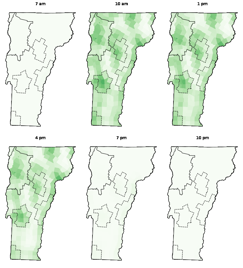
Because of the significant variation in opening and closing hours of pharmacies on Sundays and our desire to compare hourly accessibility across days of the week, we decided to run the model for every hour between 7 am and 11 pm on weekdays, Saturdays, and Sundays. Although there is minimal variation in accessibility throughout conventional 9 am to 5 pm business hours on weekdays, this approach allowed us to include time periods that are likely to pose accessibility issues to patients, while also meaningfully comparing accessibility across days of the week. This approach establishes temporal granularity, providing a comprehensive understanding of spatial and temporal accessibility dynamics within pharmacy care across Vermont by capturing fluctuations in access over multiple time points throughout the week. Through this method, we aim to comprehensively evaluate pharmacy accessibility and identify any disparities in access across both space and time within the state.
Background
Pharmacy care has recently emerged as an increasingly important part of the healthcare landscape. Pharmacies maintain a significant role in public health because of their contributions in medicine dispensing, patient consultation, vaccine delivery, and diagnostic testing, marking a continued shift from product-centered to patient-centered pharmacy care (Steeb and Ramaswamy, 2019). Recently, pharmacies have been instrumental in supporting the United States’s health and recovery throughout the COVID-19 pandemic (Grabenstein, 2022). Evidence suggests that community pharmacies are well-suited to provide preventive healthcare services due to their convenient locations and extended operational hours (San-Juan-Rodriguez et al., 2018). Pharmacies play a crucial role in ensuring equitable access to healthcare by reaching underserved individuals who lack access to other healthcare settings (San-Juan-Rodriguez et al. 2018), as well as rural residents with limited access to primary care providers (Berenbrok et al., 2020). In general, pharmacies can be particularly important for providing healthcare services in limited resource settings (Steeb and Ramaswamy, 2019).
Across the United States, rural populations tend to experience increased difficulty in accessing healthcare. Vermont has the highest proportion of its residents living in rural areas of any state in the US at 64.9% (U.S. Census Bureau, 2022). Thus, it may be important to pay attention to pharmacy care as an effective method to provide accessible healthcare services to many of Vermont's municipalities. Vermont's age demographics are additionally important when considering access to pharmacies and other healthcare services. Vermont ranks as the fourth oldest state in the US in terms of the proportion of elderly people (population 65 and over) (US Census Bureau, 2023). Older populations are more reliant on pharmacy services given their higher utilization rates of prescription medications compared to younger demographics (Martin et al.,2019). Understanding gaps in spatial accessibility to pharmacies in Vermont is especially crucial given these demographics.
Information regarding pharmacy access in Vermont is extremely sparse. The Vermont State Department of Health indicated that full-time pharmacists per 100,000 people were highest in counties with the largest urban areas, while the most rural counties, such as Essex County and Grand Isle County, had the lowest numbers of pharmacists per 100,000 (VTDOH, 2021). However, this data does not necessarily accurately reflect accessibility due to the lack of consideration of the distribution of demand (competition for services) and the necessary travel to these pharmacies, and the analysis is not at a granular enough scale to garner a meaningful understanding of variation in pharmacy accessibility.
Measuring access to healthcare has often been discussed in terms of affordability and availability, with less attention paid to spatial, or geographic, accessibility. However, there has been a notable shift in recent years towards analyzing spatial accessibility to healthcare services. Research indicates that geographic access impacts the utilization of various healthcare services, such as primary care (Arcury et al., 2005) and hospitals (Goodman et al., 1997). Specifically, studies have demonstrated that larger travel distances from pharmacies are associated with lower utilization rates (Hiscock et al., 2008).
Despite the increase in recognition of spatial methods in understanding healthcare accessibility, the literature on geographic access to pharmacy care remains limited. Of the existing literature, much has quantified access based on relatively simple methods, such as calculating pharmacy density within a geographic area (Tharumia Jagadeesan & Wirtz, 2021) or proportions of populations living within given travel distances to the nearest pharmacy (Law et al.,2011). To our knowledge, only three other studies have applied the 2SFCA or E2SFCA method to pharmacy access (Ikram et al., 2015; Wang and Ramroop, 2018; Zhou et al., 2021).
The E2SFCA method has several benefits compared to other common methods that have been used to investigate geographic accessibility to pharmacies. Unlike others, the E2SFCA method accounts for dynamics related to both supply and demand, as well as their interactions. Recent studies have started to include a temporal element into their spatial accessibility analyses, varying travel times, supply variables, and demand variables based on time (Jumadi et al., 2022; Kim and Kwon, 2022). However, we only varied our supply variables (pharmacy staffing) based on time due to the lack of granular data on travel times and real-time data on people's locations. It may be possible to gather information on how demand shifts throughout the day using mobile phone location data. Consideration of variation in travel times in spatiotemporal accessibility studies is often conducted in large metropolitan areas where variation in traffic congestion can severely impact travel times. Due to Vermont's rural nature and lack of a large metropolitan area, this consideration was not a concern in our study.
Since varying time periods can lead to significant differences in accessibility, it is important that accessibility studies of healthcare, which is often time-sensitive, consider this dimension. The inclusion of this temporal dimension has the ability to drastically improve the complexity of a spatial accessibility model, and thus the value and applicability of the conclusions. By running our analysis through various time points in a given week, we intended to elucidate some of these more complex accessibility dynamics, increasing the value of our study from a policy and healthcare planning perspective.
Materials and procedure
Computational environment
Similar to Kang et al. (2020), this study was run using CyberGIS-Jupyter. This study uses an updated software environment from the reproduction study, using Python Jupyter Notebooks in the CyberGISX environment available at https://cybergisxhub.cigi.illinois.edu/. In particular, we use the Python 3-0.9.0 Kernel running Python 3.8.12, pandas 1.3.5, geopandas 0.10.2, networkx 2.6.3 and osmnx 1.1.2.
# Import modules
import numpy as np
import pandas as pd
import geopandas as gpd
import seaborn as sns
import networkx as nx
import osmnx as ox
import re
from shapely.geometry import Point, LineString, Polygon
import matplotlib.pyplot as plt
import os
import time
import warnings
import IPython
import requests
from IPython.display import display, clear_output
from shapely.ops import nearest_points #for pharmacy_setting function
from scipy.stats import kruskal
from matplotlib import colors
from matplotlib.lines import Line2D
from matplotlib.animation import FuncAnimation
from matplotlib.colors import Normalize
from matplotlib.cm import ScalarMappable
import matplotlib.patheffects as path_effects
from tabulate import tabulate
from matplotlib.colors import ListedColormap
from mpl_toolkits.axes_grid1.anchored_artists import AnchoredSizeBar
from matplotlib.font_manager import FontProperties
from matplotlib.patches import Patch
import imageio
warnings.filterwarnings("ignore")
print('\n'.join(f'{m.__name__}=={m.__version__}' for m in globals().values() if getattr(m, '__version__', None)))
numpy==1.22.0 pandas==1.3.5 geopandas==0.10.2 seaborn==0.11.2 networkx==2.6.3 osmnx==1.1.2 re==2.2.1 IPython==8.3.0 requests==2.27.1 imageio==2.13.5
Check Directories
# Check working directory
os.getcwd()
# Use to set work directory properly
if os.path.basename(os.getcwd()) == 'code':
os.chdir('../../')
os.getcwd()
Methods
The conventional two-step floating catchment area (2SFCA) method, pioneered by Luo and Qi (2009), is a widely used approach for assessing healthcare accessibility based on service-to-population (supply-to-demand) ratios. In this method, catchment areas are defined around healthcare facilities using a threshold travel time, within which the service-to-population ratio is computed. We computed these travel times using the OSM road network's driving distances and speed limits. The accessibility at each residential location is then determined by summing up these ratios, indicating which areas are relatively more accessible compared to others. However, this method assumes equal spatial accessibility for residents within the same catchment area, which does not accurately reflect the fact that individuals are more likely to visit closer services.
The enhanced two-step floating catchment area (E2SFCA) method, pioneered by Luo and Qi (2009), addresses this limitation by considering distance decay. To do so, it incorporates multiple travel time zones (e.g., 0–10, 10–20, and 20–30 minutes) within the larger catchment area with corresponding distance weights (1, .68, and .22). This allows for a more nuanced assessment of spatial accessibility by accounting for the varying likelihood of individuals accessing facilities at different distances. The accessibility is computed as a summation of accessibility measures across each travel interval, providing a more comprehensive understanding of healthcare accessibility.
The E2SFCA method involves calculating a service-to-population ratio for each supply location (pharmacy) and aggregating these ratios for overlapping residential areas. Our service values were established by surveying pharmacies in Vermont and receiving information on the number of pharmacists and pharmacy technicians that typically work on weekdays, Saturdays, and Sundays at each location. We summed the number of pharmacists and half the technicians for these days to compute a total "service" value for each pharmacy, considering that pharmacists are relatively more important than technicians for pharmacy operations. Then, the weighted service-to-population ratios are normalized and aggregated into Vermont town geographic units using an area-weighted overlay.
In our temporally explicit model, we calculated these service-to-population ratios for weekdays, Saturdays, and Sundays differentially based on the number of pharmacists and pharmacy technicians that work on each day, as well as for different hours on each day based on operational hours of pharmacies. However, due to restrictions in our survey's ability to capture more complex staffing models (i.e. variation in staffing throughout the day) and for simplicity, the staffing levels within days were assumed to be constant for each hour of that day. Variation in accessibility between hours in a given day is demonstrated by whether a pharmacy is open, whereby zero staff are reported if it is closed, lowering the service-to-population ratio in a given catchment.
By implementing operational hours (temporal explicitness) and staffing levels into our analysis, we attempted to eliminate the limitation of assuming equal capacity of all pharmacies in other 2SFCA studies, such as Zhou et al.'s (2021) and Wang and Ramroop's (2018) spatial accessibility to pharmacies study.
Data and variables
Three main datasets were used for this study, only one of which includes primary data: 1) A retail pharmacy dataset, including the locations, hours of operations, and staffing levels of each retail pharmacy in Vermont, 2) a population dataset, and 3) a road network dataset. The list of active pharmacies was sourced from the Vermont Office of Professional Regulation (OPR) and the Homeland Infrastructure Foundation-Level Data (HIFLD) provided by the Department of Homeland Security (DHS). A list of all pharmacies within the study area was compiled by aggregating these data sources and checking them against Google Maps and OpenStreetMap (OSM). By conducting surveys, we verified the publicly available data regarding operational hours and gathered information on pharmacy staffing levels. The population dataset is sourced from the United States Census Bureau and contains information on the populations living in Vermont towns, as well as some demographic information on those towns. The road network dataset is pulled from OSM using the OSMnx package in Python.
The sole primary data source for the study includes the data we collected on pharmacies, while the secondary data sources for the study include the residential dataset and the road network data.
(1) Pharmacy Dataset
Standard Metadata
Abstract
: This dataset is primary data that was collected through surveying all VT pharmacies about their staffing levels and hours of operations. It contains information on each VT pharmacy's (117) location, hours of operations on weekdays, Saturdays, and Sundays, and the number of pharmacists and pharmacy technicians that typically work on a given day. It also includes data on the hours of operations of the 75 pharmacies within 10 miles of the VT border (NY, MA, NH). Staffing data was not collected for pharmacies outside of Vermont. Instead, staffing data was interpolated for all out-of-state pharmacies and pharmacies in Vermont for which data could not be collected. There were 192 pharmacies included in our study area in total.Spatial Coverage
: Vermont and ten miles within in Vermont state border, encompassing parts of New York, Massachusetts, and New Hampshire. Canada was excluded.Spatial Resolution
: This data specifies the specific coordinates of the pharmacy locations of interest. Resolution is not relevant.Spatial Reference System
: EPSG 6589 in order to match the results maps.Temporal Coverage
: Data was collected over the course of a couple of months, but it theoretically represents an average or typical week in the fall or early winter of 2023.Temporal Resolution
: The temporal resolution of service is hours while the temporal resolution of staffing levels is a typical work week.Lineage
: Initial pharmacy list of 127 pharmacies was downloaded from the Vermont Office of Professional Regulation (https://secure.professionals.vermont.gov/prweb/PRServletCustom?UserIdentifier=LicenseLookupGuestUser) and modified to exclude no longer active pharmacies and non-retail pharmacies. 10 pharmacies on the list were removed, totaling 117 VT pharmacies. The pharmacy locations were checked against Google Maps and a national pharmacy dataset from the Department of Homeland Security (DHS) to ensure all pharmacies in the state were included. Pharmacy locations outside of Vermont but within study area were included through querying pharmacies from OSM in QGIS, Google Maps searches, and the DHS pharmacy dataset. Pharmacies that had been closed were omitted from the data. Data on hours of operations and staffing were sourced through surveys and manually inputted by the authors. Staffing data was collected for 87% of pharmacies in VT, which was used to interpolate staffing for out-of-state pharmacies. This protocol was approved by the Middlebury College Institutional Review Board (#264).Distribution
: The majority of this dataset will be made public and downloadable on a GitHub repository. The staffing data will not be made public due to the proprietary nature of this information; however, the staffing data may be available upon request.Constraints
: We have agreed not to publicly release staffing levels of the pharmacy locations due to the proprietary nature of this data for some of the larger pharmacy chains.Data Quality
: The initial pharmacy list was checked against the DHS dataset and visualized in GIS (satellite imagery) against OpenStreetMap to ensure the correct locations of active pharmacies. We also check hours of operations posted online against what we are told during our surveys -- hours of operations incorrectly posted online were edited to match survey responses.Variables
:
Label | Definition | Type |
---|---|---|
pharmid | unique pharmacy identifier | Text |
pharmacy_name | business name | Text |
type | chain, independent, grocery, department, hospital | Text |
address | pharmacy street address | Text |
state | state in which pharmacy is located | Text |
lat | GPS coordinates. Lat | Decimal |
lon | GPS coordinates. Lon | Decimal |
week_open | opening time (24-hr) on weekdays | Integer |
week_close | closing time (24-hr) on weekdays | Integer |
sat_open | opening time (24-hr) on Saturdays | Integer |
sat_close | closing time (24-hr) operations on Saturdays | Integer |
sun_hours | opening time (24-hr) on Sundays | Integer |
sun_hours | closing time (24-hr) on Sundays | Integer |
week_pharm | Typical # pharmacists on weekday | Integer |
week_tech | Typical # pharm. techs on weekdays | Integer |
sat_pharm | Typical # pharmacists on Saturday | Integer |
sat_tech | Typical # pharm. techs on Saturdays | Integer |
sun_pharm | Typical # pharmacists on Sundays | Integer |
sun_tech | Typical # pharm. techs on Sundays | Integer |
Accuracy
: We are confident in the accuracy of the pharmacy list in Vermont. Our confidence in the out-of-state retail pharmacy locations is slightly diminished since these pharmacy locations are not based on a recent dataset from the respective states. We have confidence in the quality of the data on pharmacy staffing and hours of operations for VT pharmacies since we collected the data by surveying all pharmacies. Hours of operations for non-VT pharmacies were pulled from online. The spatial accuracy of the dataset is further confirmed as we ensured that the point coordinates for the pharmacies were within the building footprint polygon on the OSM map layer in QGIS.Domain
: The expected range of all of the pharmacy operational hours is from roughly 7 am to 10 pm. The expected range of pharmacists and technicians is from one to ten for weekdays, Saturdays, and Sundays.Missing Data Value(s)
: For any missing data on the number of pharmacists and pharmacy technicians at a given pharmacy location, the values are interpolated based on collected data for pharmacies of the same type. There is no missing data for hours of operations, as operational hours for non-surveyed out-of-state pharmacies were pulled from online.Missing Data Frequency
: We were able to collect staffing data for 102 of 117 pharmacies in Vermont.
Load and Visualize Pharmacy Data
This data contains the hours of operations and the number of pharmacists and pharmacy technicians staffed at each pharmacy. All open and close times are reported in 24-hour time. Values of -1 indicate that the pharmacy is closed.
# Read in pharmacy data
pharmacies = gpd.read_file('./data/raw/public/pharmacy/pharmacies_df.gpkg')
pharmacies.head()
pharmid | pharmacy_name | type | address | state | lat | lon | week_open | week_close | sat_open | sat_close | sun_open | sun_close | geometry | |
---|---|---|---|---|---|---|---|---|---|---|---|---|---|---|
0 | VT99 | Walgreen Eastern Co., Inc. d/b/a Walgreens #18325 | chain | 30 Shelburne Shopping Park, Shelburne, VT | VT | 44.379262 | -73.224989 | 9.0 | 19.0 | -1.0 | -1 | -1.0 | -1 | POINT (-73.22499 44.37926) |
1 | VT98 | WALGREENS #19795 | chain | 133 N Main St Ste 23, Saint Albans, VT | VT | 44.814168 | -73.082604 | 9.0 | 19.0 | 9.0 | 18 | 9.0 | 17 | POINT (-73.08260 44.81417) |
2 | VT97 | WALGREENS #17747 | chain | 201 Route 7 S, Milton, VT | VT | 44.682189 | -73.112042 | 9.0 | 19.0 | 9.0 | 18 | -1.0 | -1 | POINT (-73.11204 44.68219) |
3 | VT96 | Walgreens #19346 | chain | 221 Main St, Enosburg Falls, VT | VT | 44.905772 | -72.806612 | 9.0 | 19.0 | 9.0 | 18 | -1.0 | -1 | POINT (-72.80661 44.90577) |
4 | VT95 | Walgeens #17183 | chain | 1184 Prim Rd Ste 2, Colchester, VT | VT | 44.537734 | -73.247286 | 9.0 | 20.0 | 9.0 | 18 | 9.0 | 17 | POINT (-73.24729 44.53773) |
Map pharmacies and their hours.
pharmacies.explore()
# staffing_interpolated.csv is confidential.
# with permission from researchers, download from OSF at https://osf.io/download/b956m/
#if not os.path.exists("./data/raw/private/staffing_interpolated.csv"):
# print("Loading pharmacy staffing levels", flush=True)
# url = 'https://osf.io/download/b956m/'
# r = requests.get(url, allow_redirects=True)
# open('./data/raw/private/staffing_interpolated.csv', 'wb').write(r.content)
# Load pharmacy staffing data
pharm_staffing = pd.read_csv('./data/raw/private/staffing_interpolated.csv')
pharm_staffing.head()
# Join private staffing data to pharmacies dataset (locations, hours of operations, etc.)
pharmacies_df = pd.merge(pharmacies, pharm_staffing, on='pharmid', how = 'left')
pharmacies_df
(2) Population Dataset
Standard Metadata
Abstract
: Secondary data pulled from the US Census Bureau, containing information on demographics of county subdivisions (towns). This data also contains information from the Census defining towns as metropolitan or micropolitan.Spatial Coverage
: Vermont.Spatial Resolution
: County subdivisions (towns)Spatial Reference System
: NATemporal Coverage
: 2018-2022 ACS (5-year estimates)Temporal Resolution
: NA.Lineage
: This data is downloaded using the TidyCensus package in R. This allowed for necessary data to be easily downloaded with the corresponding GEOID (FIPS) for each town in our study area. The R code to retrieve this data is in the procedure/code folder. Only total population and age variables were selected, as these are the only demographic data necessary for our study. The metropolitan and micropolitan classifications are downloaded separately and appended to the population dataset in this notebook.Distribution
: The total population and age data is downloadable from the US Census Bureau ACS page (https://data.census.gov/table?g=040XX00US50$0600000) and the town classifications are downloadable at: https://www2.census.gov/programs-surveys/metro-micro/geographies/reference-files/2020/delineation-files/ (list 3).Constraints
: US Census Bureau data is in the public domain.Data Quality
: Census provides data on margins of error.Variables
:
Label | Definition | Type | Accuracy | Domain | Missing Data Value(s) | Missing Data Frequency |
---|---|---|---|---|---|---|
GEOID | Town unique identifier | Integer | NA | NA | NA | NA |
total_pop | Total population in a town | Integer | Defined by Census | 0 - ~45,000 | NA | NA |
subdivision_name | Name of county subdivision (town) | Text | NA | NA | NA | NA |
elderly_pop | Total elderly population in a town | Integer | Defined by Census | 0 - ~1,000 | NA | NA |
percent_elderly | Percent elderly residents in a town | Decimal | Defined by Census | 0% - ~50% | NA | NA |
geometry | Geo data for each town in study area | Text | NA | NA | NA | NA |
necta | Classified as metropolitan or micropolitan | Text | Defined by Census | NA | NaN | Frequent because missing data means town is rural |
Load and Visualize Population Data
This dataset contains population data by town for all states in our study area (VT, NH, MA, NY). VT towns have data on micropolitan/metropolitan classification and elderly population.
# Read in population data by town
population_df = gpd.read_file('./data/raw/public/population/tidycensus_population.gpkg')
# Read in metropolitan / micropolitan classifications (NECTAS)
nectas_df = gpd.read_file('./data/raw/public/population/nectas.csv')
# Join NECTAS classifications to population data with subdivision and county FIPS
pop_df = pd.merge(population_df, nectas_df[['fips_subdivision', 'necta', 'fips_county', 'fips_state']], on=['fips_subdivision','fips_county', 'fips_state'], how = 'left')
# Save as geopackage into public/derived
pop_df.to_file('./data//derived/public/pop_data.gpkg', driver='GPKG')
pop_df.head()
# All geometries for which we have obtained population data
pop_df.plot()
<AxesSubplot:>
(3) OpenStreetMap Roads for Vermont and Surroundings
Standard Metadata
Abstract
: This is a graph data structure representing roads and streets in Vermont and surrounding areas. The data is derived from OpenStreetMap via the Overpass API and OSMnx python package.Spatial Coverage
: The state of Vermont and a 64373.8 meter (40 mile) buffer around the state.Spatial Resolution
: The spatial resolution varies by region and feature. Distances are calculated with the full spatial resolution of the dataset, but the graph model is simplified to vertices at intersections and dead ends only.Spatial Reference System
: WGS 1984 geographic coordinate system (EPSG:4326)Temporal Coverage
: Data was queried on 24-1-2024Temporal Resolution
: Data represents a snapshot of the OpenStreetMap database at a moment in time. Data currency varies by region and feature, depending on how recently any OpenStreetMap users have digitized or updated the map.Lineage
: See code for creation at procedure/code/00_road_network.ipynb. OpenStreetMap data is volunteered by users, and lineage varies on a feature-by-feature basis. OSMnx software version 1.8.1 was used to query the data from OpenStreetMap using the Overpass API with the queryox.graph_from_place('Vermont', network_type='drive', buffer_dist=64373.8)
. By default, this saves data in the WGS 1984 geographic coordinate system (EPSG:4326), calculates the distance of all lines, and simplifies the road network by combining road segments between intersections into a single edge. The road network is then saved as a NetworkX graph data structure in a .graphml file.Distribution
: This graph dataset is stored on OSF at https://osf.io/bwrmu/ while the original data is stored on OpenStreetMap and distributed via the Overpass API https://wiki.openstreetmap.org/wiki/Overpass_APIConstraints
: The graph dataset is published with a BSD 3-Clause license, while the original OpenStreetMap data is published with the Open Data Commons Open Database License (https://opendatacommons.org/licenses/odbl/). The data is (c) OpenStreetMap Contributors, and this copyright and license information must be attached to any public uses or distributions of the data.Data Quality
: Data has been checked for speed attribute completeness. Routing errors and resulting service areas calculated on the graph from hospitals were checked for topological errors and consistency, resulting in discovery of four erroneous "dead-ends" where one-way access roads terminated in parking areas. These four dead-end nodes are removed from the analysis code so that routes start on the correct one-way exit from parking areas.Variables
:
Label | Alias | Definition | Type | Accuracy | Domain | Missing Data Value(s) | Missing Data Frequency |
---|---|---|---|---|---|---|---|
osmid | osmid | unique OpenStreetMap identifier | long integer | n/a | n/a | none | none |
highway | highway | highway key from OpenStreetMap with values indicating highway type | text | unknown | residential, tertiary, secondary, primary, unclassified, trunk, etc. See https://wiki.openstreetmap.org/wiki/Key:highway | no value recorded | 194,089 of 577,399 edges missing highway type |
oneway | oneway | road is for one-way travel only | text representing boolean | unknown | {true, false} | n/a | n/a |
reversed | reversed | road direction is opposite the sequence of coordinates | text representing boolean | unknown | {true, false} | n/a | n/a |
length | length | length in meters | decimal | geodesic calculation with epsg 4326 | unknown | n/a | none |
| maxspeed | maximum speed limit | maximum speed limit (assumed kph unless other units are written) | text composed of an integer, integer with speed limit, or list of speeds | unknown | one | no value recorded | 411,768 of 577,399 edges missing speed limit |
Load the Road Network
If Vermont_Network_Buffer.graphml
does not already exist, this cell will query the road network from OpenStreetMap.
Each of the road network code blocks may take a few mintues to run.
%%time
# To create a new graph from OpenStreetMap, delete or rename the graph file (if it exists)
# AND set OSM to True
# This is more likely to work on a local computer than CyberGISX
# This network was created on Windows with Python 3.12.1 and osmnx 1.8.1 on 2024-01-24
# using the 00_road_network.ipynb script
OSM = False
# Define the place name for Vermont
place_name_vermont = 'Vermont, USA'
roads_path = "./data/raw/private/osm_roads.graphml"
# if buffered street network is not saved, and OSM is preferred, generate a new graph from OpenStreetMap and save it
if not os.path.exists(roads_path) and OSM:
print("Loading buffered Vermont road network from OpenStreetMap. Please wait... runtime may exceed 9min...", flush=True)
G = ox.graph_from_place(place_name_vermont, network_type='drive', buffer_dist=64373.8)
print("Saving road network to", roads_path, " Please wait...", flush=True)
ox.save_graphml(G, roads_path)
print("Data saved.")
# otherwise, if buffered street network is not saved, download graph from the OSF project
elif not os.path.exists(roads_path):
print("Downloading buffered Vermont road network from OSF...", flush=True)
url = 'https://osf.io/download/bwrmu/'
r = requests.get(url, allow_redirects=True)
print("Saving road network to", roads_path, " Please wait...", flush=True)
open(roads_path, 'wb').write(r.content)
# load the saved network graph
if os.path.exists(roads_path):
print("Loading road network from", roads_path, "Please wait...", flush=True)
G = ox.load_graphml(roads_path)
print("Data loaded.")
else:
print("Error: could not load the road network from file.")
Loading road network from ./data/raw/private/osm_roads.graphml Please wait... Data loaded. CPU times: user 1min 21s, sys: 5.51 s, total: 1min 27s Wall time: 1min 41s
Plot the Road Network
%%time
ox.plot_graph(G, node_size = 1, bgcolor = 'white', node_color = 'black', edge_color = "#333333", node_alpha = 0.2, edge_linewidth = 0.5)
CPU times: user 1min 8s, sys: 2.67 s, total: 1min 11s Wall time: 1min 17s
(<Figure size 576x576 with 1 Axes>, <AxesSubplot:>)
Check speed limits and highway types
Display all the unique speed limit values and count how many network edges (road segments) have each value. We will compare this to our cleaned network later.
%%time
# Turn network edges into a geodataframe
edges = ox.graph_to_gdfs(G, nodes=False, edges=True)
# Count frequency of each speed value
speed_values = edges['maxspeed'].value_counts()
# Ouput number of edges and frequences of speed values
print(str(len(edges)) + " edges in graph")
print(speed_values.to_string())
Display all the unique highway types, which are used to impute the speed limits for each category of highway.
# view all highway types
print(edges['highway'].value_counts())
Process the road network
Impute speed limits with add_edge_speeds
function.
%%time
ox.speed.add_edge_speeds(G)
Calculate travel time with the add_edge_travel_times
function.
%%time
ox.speed.add_edge_travel_times(G)
Add a point geomerty to each node in the graph, to facilitate constructing catchment area polygons later on.
%%time
# Create point geometries for each node in the graph, to make constructing catchment area polygons easier
for node, data in G.nodes(data=True):
data['geometry']=Point(data['x'], data['y'])
%%time
# Turn network edges into a geodataframe
nodes,edges = ox.graph_to_gdfs(G, nodes=True, edges=True)
# Count frequency of each speed value
speed_values = edges['speed_kph'].value_counts()
# Ouput number of edges and frequences of speed values
print(str(len(edges)) + " edges in graph")
print(speed_values.to_string())
Unplanned deviation: We discovered four errors in which one-way parking lot entrance lanes terminated without any topological connection to routes through the parking lot our out the exit lane. In the unplanned deviation below, we remove the four dead-end nodes such that the pharmacy locations join the network on the exit lane rather than entrance lane, and proceed to calculate travel routes correctly.
# Drop four dead-end nodes for parking lot entrances
nodes.drop([205007938, 5976921845, 204567135, 61755372], inplace = True)
Speeds have been imputed and converted to kilometers per hour.
# calculate a color scheme for edges based on speed
ec = ox.plot.get_edge_colors_by_attr(G, attr="speed_kph", cmap='YlOrRd')
# plot edge speeds
fig, ax = ox.plot_graph(G, node_size=0, edge_color=ec, bgcolor="white")
The graph of speed limits looks accurate, with local roads at low speeds and state and federal highways at higher speeds.
Data transformations
The data transformations taken in this study primarily occur in our primary data. Minimal transformations were made to the population and road network data sets. The population dataset is an aggregate of two data frames: one with total population and percent elderly in county subdivisions, and one with metropolitan or micropolitan class at the county subdivision level, so these datasets were merged.
The initial pharmacy list encompassing all retail pharmacies in Vermont and within ten miles of the Vermont border was derived from data from the Vermont Office of Professional Regulation (OPR) and checked against a dataset of pharmacy locations from the Department of Homeland Security (DHS) in order to increase our confidence in the pharmacy list. The DHS data set included the geolocations for pharmacies across the United States, while the OPR dataset provided addresses for each pharmacy licensed in Vermont. Using the MMQGIS plugin in QGIS, all pharmacies in the OPR dataset were geolocated. A 100 meter buffer was then placed around these points to account for some error in geolocation as well as the possibility for variation in the placement of the point within a given pharmacy building footprint. The DHS pharmacies that were located within these buffers were merged. All the DHS pharmacy locations that fell outside of the OPR pharmacy buffers were then manually checked against Google Maps to confirm whether they were active and separate retail pharmacies from those in the OPR dataset. All permanently closed pharmacies and non-retail pharmacies were omitted from the DHS dataset, which remedied all the discrepancies between the two datasets. There were no active separate retail pharmacies in the DHS dataset that were missed in the OPR dataset (not within OPR buffer). Thus, we have high confidence in the data accuracy for active Vermont retail pharmacies as a result of this method. The initial raw OPR list contained 127 pharmacies, and we included only 117 Vermont pharmacies in our analysis.
In order to locate the out-of-state pharmacies of interest, a 10 mile buffer was created around the Vermont state boundary and all DHS pharmacies that intersected with this buffer were selected. This includes pharmacies in New York, Massachusetts, and New Hampshire. A ten mile buffer was chosen since this geographic extent includes the nearby major out-of-state towns that are likely to service Vermont residents, including Lebanon, NH, North Adams, MA, Greenfield MA, Plattsburgh, NY, and Keene, NH. There were no urban centers that were excluded and within a reasonable distance of the Vermont border. These locations were checked against queried pharmacy locations from OpenStreetMap (OSM), using the QuickOSM plugin in QGIS, and manually checked against pharmacy locations on Google Maps. Ultimately, a list of out-of-state pharmacies was compiled through repeated Google Maps searches along the outside of the Vermont border. Through this triangulation, permanently closed pharmacies and non-retail pharmacies were removed from the list, and any extra pharmacies that were present on Google Maps or OSM were checked against each other and added to the out-of-state list. 75 out-of-state retail pharmacies were included. This was in the range of the DHS dataset for out-of-state pharmacies in our study area (78) and far more than the number of queried pharmacies from OSM in GQIS using the QuickOSM plugin (45). This makes sense considering the inaccuracy and outdated nature of the DHS and OSM datasets. Our confidence in the out-of-state retail pharmacy locations is slightly diminished since these pharmacy locations are not based on a recent dataset from the respective states. However, the out-of-state locations are as not significant as Vermont locations and are primarily included to minimize the edge effects of such an analysis. As such, out-of-state pharmacy locations were not surveyed to collect hours of operations or staffing data; instead, their hours were pulled from online.
Once the list of in-state pharmacies was confirmed and the list of out-of-state pharmacies was compiled, these datasets were aggregated and variable columns for staffing and hours of operations were created. A column for the number of pharmacists, number of pharmacy technicians, and opening and closing hours was created for weekdays, Saturdays, and Sundays. For all hours of operation, the opening and closing times were reported on the 24-hour clock. If the pharmacy is closed on Saturday or Sunday, the values for staffing were reported as zero, and the open and close hours were reported as -1. Pharmacies that opened or closed at the half-hour mark were denoted in our data frame with a 0.5; However, because the variation in accessibility was unlikely to be significant in intervals under one hour, we did not calculate accessibility for half hours. For example, a pharmacy that opened at 8:30 am was not included in the accessibility measurement until 9 am, and one that closed at 5:30 pm was not included in the 5 pm accessibility calculation.
Unplanned Deviation: There was missing data for staffing levels for 15 pharmacy locations in our VT study area due to non-response from survey participants. Therefore, we assumed that on-line pharmacy hours for the locations were correct and we interpolated staffing levels based on weekday, Saturday, and Sunday averages of the collected data for the same pharmacy type (chain vs independent). During our data collection process, we originally classified pharmacies as chain, grocery, or independent, but ultimately decided to group grocery and chain as there were relatively few grocery locations and their staffing models appeared to be similar. For independent pharmacies, the average number of pharmacists and technicians was 2 and 4 on weekdays, 1 and 2 on Saturdays, and 1 and 2 on Sundays. For chain pharmacies, these values were 1 and 2 on weekdays, 1 and 1 on Saturdays, and 1 and 1 on Sundays. We reached out to regional pharmacy managers of large pharmacy chains attempting to collect staffing data for multiple locations.
Unplanned Deviation: One pharmacy chain regional manager provided budgeted weekly hours for pharmacists and pharmacy technicians. We combined this data with operational hours of their pharmacy locations to estimate staffing levels.
Unplanned Deviation: In order to limit the time of our data collection, we did not collect any staffing data for pharmacies outside of Vermont. Instead, we used the interpolated values from Vermont pharmacies, since the accuracy of staffing data for these pharmacies is not as important due to the fact that they were included to minimize edge effects in our analysis. We adjusted the staffing data for one outlier, where a location reported an unusually high number of pharmacy technicians (15) working on weekdays. Recognizing this figure as an outlier, we adjusted it by considering the ratio between the reported number of weekend technicians (4) and weekday technicians, as well as the standard ratio between pharmacists and pharmacy technicians, resulting in an adjustment to 7 weekday technicians.
Analysis
This section implements the enhanced 2-step floating catchment area (E2SFCA) method.
We adapted code originally developed by Kang et al. (2020) to calculate distance-weighted catchment areas for each hospital. Prior to this study, Holler et al. (2023) improved the efficiency, legibility and accuracy of the code in a reproduction study. In this study, we have adapted the method to calculate accessibility for pharmacies and extended it to consider accessibility over time. First, we create a dictionary (with a node and its corresponding drive time from the pharmacy) of all nodes within a 30 minute drive time (using single_source_dijkstra_path_length function). From here, two more dictionaries are constructed by querying the original one (20 min and 10 min). From these dictionaries, single part convex hulls are created for each drive time interval and appended into a single list (one list with 3 polygon geometries for each unique pharmacy). Within the list, the polygons are differenced from each other to produce three catchment areas (not overlapping).
Creating catchment areas
Runs spatial join to find a unique nearest node for each pharmacy.
nodes_osmid = gpd.GeoDataFrame(nodes[["geometry"]]).reset_index()
# print(nodes_osmid.head())
pharmacies_osm = gpd.sjoin_nearest(pharmacies_df, nodes_osmid, distance_col="distances")
#rename column from osmid to nearest_osm, so that it works with other code
pharmacies_osm = pharmacies_osm.rename(columns={"osmid": "nearest_osm"})
Three different catchment areas are created for each pharmacy using convex hulls, represented by the time it takes to drive 10, 20, and 30 minutes from a given pharmacy. These drive times are weighted differently, with the 10-minute catchment carrying the most weight and the 30-minute catchment carrying the least weight.
distances = [600, 1200, 1800] # Distances in travel time (seconds!) (10 min, 20 min, 30 min)
weights = [1.0, 0.68, 0.22] # Relative weights of 10 minute catchment, 20 minute catchment, and 30 minute catchment
# initialize catchment list, composed of 3 empty geodataframes for 3 distance bands
catchments = []
for distance in distances:
catchments.append(gpd.GeoDataFrame())
# initialize results geodataframe to store final catchment areas
results = gpd.GeoDataFrame(columns = ["geometry","pharmid","weight"], crs = "EPSG:4326", geometry = "geometry")
# calculate catchment areas
print("Working on pharmacy:")
for ind in pharmacies_osm.index:
print(str(ind + 1) + "/" + str(len(pharmacies_osm)), end = '\r')
# print(pharmacies_osm['pharmid'][ind], end=' ')
## CREATE DICTIONARIES ##
# create dictionary of nearest nodes
nearest_nodes_30 = nx.single_source_dijkstra_path_length(G, pharmacies_osm['nearest_osm'][ind], distances[2], "travel_time") # creating the largest graph from which 10 and 20 minute drive times can be extracted from
# extract values within 20 and 10 (respectively) minutes drive times
nearest_nodes_20 = dict()
nearest_nodes_10 = dict()
for key, value in nearest_nodes_30.items():
if value <= distances[1]:
nearest_nodes_20[key] = value
if value <= distances[0]:
nearest_nodes_10[key] = value
## CREATE POLYGONS FOR 3 DISTANCE CATEGORIES (10 min, 20 min, 30 min) ##
# 30 MIN
# If the graph already has a geometry attribute with point data,
# this line will create a GeoPandas GeoDataFrame from the nearest_nodes_30 dictionary
points_30 = gpd.GeoDataFrame(gpd.GeoSeries(nx.get_node_attributes(G.subgraph(nearest_nodes_30), 'geometry')))
# This line converts the nearest_nodes_30 dictionary into a Pandas data frame and joins it to points
# left_index=True and right_index=True are options for merge() to join on the index values
points_30 = points_30.merge(pd.Series(nearest_nodes_30).to_frame(), left_index=True, right_index=True)
# Re-name the columns and set the geodataframe geometry to the geometry column
points_30 = points_30.rename(columns={'0_x':'geometry','0_y':'z'}).set_geometry('geometry')
# Create a convex hull polygon from the points
polygon_30 = gpd.GeoDataFrame(gpd.GeoSeries(points_30.unary_union.convex_hull))
polygon_30 = polygon_30.rename(columns={0:'geometry'}).set_geometry('geometry')
polygon_30["weight"] = weights[2]
# 20 MIN # 1200 seconds!
# Select nodes less than or equal to 20
points_20 = points_30.query("z <= " + str(distances[1]))
# Create a convex hull polygon from the points
polygon_20 = gpd.GeoDataFrame(gpd.GeoSeries(points_20.unary_union.convex_hull))
polygon_20 = polygon_20.rename(columns={0:'geometry'}).set_geometry('geometry')
polygon_20["weight"] = weights[1]
# 10 MIN # 600 seconds!
# Select nodes less than or equal to 10
points_10 = points_30.query("z <= " + str(distances[0]))
# Create a convex hull polygon from the points
polygon_10 = gpd.GeoDataFrame(gpd.GeoSeries(points_10.unary_union.convex_hull))
polygon_10 = polygon_10.rename(columns={0:'geometry'}).set_geometry('geometry')
polygon_10["weight"] = weights[0]
# Clip the overlapping distance ploygons (create two donuts + hole)
polygon_30_hole = gpd.overlay(polygon_30, polygon_20, how ="difference")
polygon_20_hole = gpd.overlay(polygon_20, polygon_10, how ="difference")
# Create dataframe combining polygon_10, polygon_20, polygon_30
polygons = pd.concat([polygon_10, polygon_20_hole, polygon_30_hole])
polygons.set_crs(crs="EPSG:4326", inplace = True)
# polygons = pd.concat([polygon_10, polygon_20, polygon_30])
# polygons.set_crs(crs="EPSG:4326", inplace = True)
polygons_gdf = polygons
polygons_gdf["pharmid"] = pharmacies_osm['pharmid'][ind]
#polygons_gdf["weight"] = weights
results = pd.concat([results, polygons_gdf])
The interactive map below shows the three catchment areas for each pharmacy in our study area. We check for completeness by counting the catchment areas and dividing by the total number of pharmacies, expecting a value of 3 catchment areas per pharmacy.
print(len(results) / 192) # Value of 3.0 confirms all pharmacies, since there are 192 pharmacies in our study area and 3 polygons per pharmacy
3.0
results.explore("weight", categorical=True, cmap='GnBu', style_kwds={'fillOpacity': 0.3})
# try results.explore("weight")
Service-to-population ratio calculations
To begin the process of calulating service-to-population ratios, town areas must be calculated since this is the final geographic unit we want to display our results in. This code calculates the areas where catchment areas overlap with different town geometries (fragments), and then estimates the population within these fragments by assessing the proportion of each town covered by a specific fragment. Next, these fragments are assigned weights based on the distance to a pharmacy location, culminating in an estimated population that may use services in a given pharmacy location.
# Change CRS to match prior to analysis, should be mapped in VT State Plane projection
results.to_crs("EPSG:6589", inplace = True)
pop_df.to_crs("EPSG:6589", inplace = True)
# Calculate town areas
pop_df['town_area'] = pop_df.geometry.area
#display(pop_df)
# Run the overlay to find intersection of fragments (fragments are where each individual catchment area overlaps with a different town geometry)
fragments = gpd.overlay(pop_df, results, how = 'intersection')
# Calculate fragment areas
fragments['frag_area'] = fragments.geometry.area
# Calculate area ratios to see how much of a town is covered by the given fragment --> used to estimate the population in that fragment
fragments['area_ratio']= fragments['frag_area'] / fragments['town_area']
# Calculate fragment value by multiplying area_ratio by distance weight
fragments['value'] = fragments['weight'] * fragments['area_ratio']
# Calculate population served in each fragment
fragments['pop_value'] = fragments['total_pop']*fragments['value']
fragments.head()
Next, a value for the total population served by each pharmacy is calculated by aggregating all the fragments within a given pharmacy catchment. Service-to-population ratios will ultimately be aggregated into Vermont municipalities.
# Sum population served per pharmacy
sum_values = fragments[["pharmid","pop_value"]]
sum_values = sum_values.groupby(by = ['pharmid']).sum('pop_value')
sum_values.rename(columns={'pop_value': 'total_value'}, inplace = True)
sum_values.head()
# Join summed values by pharmacy to pharmacies_df
pop_join = sum_values.merge(pharmacies_df, on='pharmid', how = 'left')
pd.set_option('display.max_columns', None)
# Only display this data for testing. It reveals confidential information at the pharmacy level.
# pop_join.head()
Then, the number of pharmacists and pharmacy technicians that work at each pharmacy is derived, and service-to-population ratios can be calculated by dividing this service value by the population value (total_value) for a pharmacy. An individual service-to-population ratio is derived for each hour on weekdays, Saturdays, and Sundays, as well as these days generally. The ratio for entire days represents a point in the day when all pharmacies are open, between the time when the last pharmacy opens and the first pharmacy closes (all pharmacists and technicians are working).
# Calculate number of staff that work at each pharmacy
# Weekday
pop_join['week_staff'] = pop_join['week_pharm'] + 0.5 * pop_join['week_tech']
#Saturday
pop_join['sat_staff'] = pop_join['sat_pharm'] + 0.5 * pop_join['sat_tech']
# Sunday
pop_join['sun_staff'] = pop_join['sun_pharm'] + 0.5 * pop_join['sun_tech']
# Calculate service to pop ratio for each pharmacy for Weekdays, Saturdays, and Sundays between 7am-11pm
def calculate_sp_ratios(pop_join, day_type):
pop_join[f'sp_ratio_{day_type}'] = pop_join[f'{day_type}_staff'] / pop_join['total_value']
for hour in range(7, 24):
pop_join[f'sp_ratio_{hour}{day_type}'] = np.where((pop_join[f'{day_type}_open'] <= hour) & (pop_join[f'{day_type}_close'] >= hour),
pop_join[f'{day_type}_staff'] / pop_join['total_value'],
np.nan)
# Weekday
calculate_sp_ratios(pop_join, 'week')
# Saturday
calculate_sp_ratios(pop_join, 'sat')
# Sunday
calculate_sp_ratios(pop_join, 'sun')
# Only display this data for testing. It reveals confidential information at the pharmacy level.
# pop_join.head()
Since our desired final result will be represented in county subdivisions, we do not need to recalculate network distances and catchments. Instead, we can join our service to population ratio data back to the fragments used above.
# Join to the fragments df
frag_join = fragments.merge(pop_join, on = 'pharmid', how = 'left')
# Only display this data for testing. It reveals confidential information at the pharmacy level.
# frag_join.head()
The service-to-population ratios for each fragment must be multiplied by the area-weight and distance weights once again. Then, all of these ratios for the fragments are summed within a county subdivision (GEOID) to create an accessibility measure for each town.
Unplanned Deviation:
An earlier report did not apply the area weight to this second step of the two-step floating catchment method.
In this version, we multiply the service to population ratios by value
, which is the distance weight multiplied by the area weight.
# Calculate weighted service to population ratio for each slice of time (weight correspond to distance from the pharmacy still)
frag_join['sp_weighted_w'] = frag_join['sp_ratio_week'] * frag_join['value']
frag_join['sp_weighted_s'] = frag_join['sp_ratio_sat'] * frag_join['value']
frag_join['sp_weighted_su'] = frag_join['sp_ratio_sun'] * frag_join['value']
def calculate_weighted_sp_ratios(frag_join, day_type):
for hour in range(7, 24):
frag_join[f'sp_weighted_{hour}{day_type}'] = frag_join[f'sp_ratio_{hour}{day_type}'] * frag_join['value']
# Weekday
calculate_weighted_sp_ratios(frag_join, 'week')
# Saturday
calculate_weighted_sp_ratios(frag_join, 'sat')
# Sunday
calculate_weighted_sp_ratios(frag_join, 'sun')
# Make all NaN values 0, since these values represent 0 access
frag_join.fillna(0, inplace = True)
# Sum weighted service to population ratio by town
accessibility_towns = frag_join.groupby('GEOID').sum()
accessibility_towns.head()
Lastly, these accessibility measures are rescaled to an estimate of pharmacist-equivalent staff (one pharmacist or two pharmacy tecnicians) per 10,000 people so that they are interpretable, whole numbers. This allows for easier comparison between towns.
#Normalize (multiply by large constant)
#Full Days
accessibility_towns['access_w'] = accessibility_towns['sp_weighted_w']*10000
accessibility_towns['access_s'] = accessibility_towns['sp_weighted_s']*10000
accessibility_towns['access_su'] = accessibility_towns['sp_weighted_su']*10000
def calculate_accessibility_times(accessibility_towns, day_type):
for hour in range(7, 24):
accessibility_towns[f'access_{hour}{day_type}'] = accessibility_towns[f'sp_weighted_{hour}{day_type}'] * 10000
# Weekday times
calculate_accessibility_times(accessibility_towns, 'week')
# Saturday times
calculate_accessibility_times(accessibility_towns, 'sat')
# Sunday times
calculate_accessibility_times(accessibility_towns, 'sun')
#Select just access columns
accessibility_towns = accessibility_towns[[col for col in accessibility_towns.columns if col.startswith('access')]]
accessibility_towns.head()
This output displays an interactive map with all of the accessibility scores for each day and hour by county subdivisions. The results appear acurate.
# Join back to geometries in pop_df for mapping. Pop_df contains town geometries
mapping_df = pd.merge(accessibility_towns, pop_df[['GEOID', 'geometry', 'fips_state', 'necta', 'pct_elderly']], on='GEOID', how='left')
mapping_df = mapping_df[mapping_df['fips_state'].isin(['50'])]
mapping_df = gpd.GeoDataFrame(mapping_df, crs="EPSG:6589", geometry='geometry')
mapping_df.explore("access_w", tooltip=["access_w", "access_s", "access_su"], cmap="Greens", scheme='Quantiles', k=6, legend_kwds={'scale':False}) # View geometries of interest with weekday, sat, sun summaries
Results
Study Area
First, we calculate population density of each county subdivision and report the number of county subdivisions per NECTA category.
# Prepare pharmacies for mapping
pharmacies_df.to_crs("EPSG:6589", inplace = True) # Match CRS for Vermont
pharmacies_map = pharmacies_df[pharmacies_df['state'] == 'VT']
# Replace NaN values in 'necta' column with 'Rural'. All towns that are not metropolitan or micropolitan are rural.
mapping_df['necta'].fillna('Rural', inplace=True)
# Replace 'Metropolitan NECTA' and 'Micropolitan NECTA' with 'Metropolitan' and 'Micropolitan', respectively
mapping_df['necta'] = mapping_df['necta'].replace({'Metropolitan NECTA': 'Metropolitan', 'Micropolitan NECTA': 'Micropolitan'})
necta_summary = mapping_df[['necta', 'GEOID']].groupby("necta").count()
necta_summary.rename(columns={"GEOID": "N"}, inplace=True)
print(necta_summary)
N necta Metropolitan 35 Micropolitan 48 Rural 172
Select county subdivisions in Vermont and calculate population density. Select pharmacies in Vermont and transform into into Vermont State Plane system.
# Calculate population denisty by town
popdensity_df = pop_df.copy()
popdensity_df = popdensity_df[popdensity_df['fips_state'].isin(['50'])]
popdensity_df.to_crs("EPSG:6589", inplace = True)
popdensity_df['town_area_km2'] = popdensity_df['town_area'] / 10**6
popdensity_df['pop_density'] = popdensity_df['total_pop']/popdensity_df['town_area_km2']
popdensity_df['pop_density'] = popdensity_df['pop_density'].replace([np.inf, -np.inf], 0) #make inf values zero since they arise from total_pop = 0
Figure 1: Mapping town types, population density, and pharmacy locations in VT
# Custom color map for pop density
base_cmap = plt.get_cmap('Blues')
num_colors = 256
custom_colors = []
for i in range(num_colors):
color = colors.rgb_to_hsv(base_cmap(i)[:3]) # Convert RGB to HSV
color[1] *= 0.7 # Reduce saturation by one third
custom_colors.append(colors.hsv_to_rgb(color)) # Convert back to RGB
custom_cmap = colors.LinearSegmentedColormap.from_list("custom_blues", custom_colors, N=num_colors)
# Map Population Density
fig1, ax = plt.subplots(figsize=(12.3, 10.8))
popdensity_df.plot(column='pop_density', scheme = 'jenkscaspallforced',k=5, cmap=custom_cmap, legend = False, ax=ax)
metropolitan_df = mapping_df[mapping_df['necta'] == 'Metropolitan']
micropolitan_df = mapping_df[mapping_df['necta'] == 'Micropolitan']
metropolitan_boundary = metropolitan_df.dissolve(by='necta')['geometry'].boundary
micropolitan_boundary = micropolitan_df.dissolve(by='necta')['geometry'].boundary
# Plot only the merged exterior boundaries of the 'Metropolitan NECTA' group
metropolitan_boundary.plot(ax=ax, color='black', linewidth=1.5)
# Plot only the merged exterior boundaries of the 'Micropolitan NECTA' group
micropolitan_boundary.plot(ax=ax, color='black', linestyle = 'dashed', linewidth=1.5)
vt_boundary = popdensity_df.dissolve().boundary
vt_boundary.plot(ax=ax, color='black', linewidth=.75)
# Legend
legend_elements = [
Line2D([0], [0], color='black', lw=2, label='Metropolitan'),
Line2D([0], [0], color='black', lw=2, linestyle= 'dashed', label='Micropolitan'),
Line2D([0], [0], marker='o', color='w', markerfacecolor='white', markeredgecolor='black', markersize=9, label='Pharmacy')
]
pd_colorbar = plt.cm.ScalarMappable(cmap=custom_cmap, norm=plt.Normalize(vmin=0, vmax=2046.6))
cbar = plt.colorbar(pd_colorbar, shrink = .38, pad=.001, label = 'Population Density (person/km^2)', location="bottom")
ax.legend(handles=legend_elements, loc='lower right', fontsize=10, bbox_to_anchor=(.95,.2))
# Plot pharmacy locations
pharmacies_map.plot(ax=ax, marker='o', facecolor='white', edgecolor='black', markersize=50, label='VT Pharmacies', legend = True)
plt.text(0.22, 0.71, 'Burlington', transform=ax.transAxes, size=11, weight="bold", color='white',
path_effects=[path_effects.Stroke(linewidth=2, foreground='black'), path_effects.Normal()])
#fig.patch.set_edgecolor('black') #Border
#fig.patch.set_linewidth(2)
plt.axis('off')
plt.show()
#Export figure to results/figures
fig1.savefig("./results/figures/figure1.jpg", dpi=300)
Figure 1. Vermont study area with population density and pharmacy locations across the state. Metropolitan and micropolitan towns are outlined.
Our study area included 117 retail pharmacies in Vermont and 75 out-of-state retail pharmacies. One group of county subdivisions is classified as metropolitan, known as the Burlington Metropolitan Area, totaling 35 metropolitan towns, while four other groups of county subdivisions in Vermont are classified as micropolitan, totaling 48 micropolitan towns (Figure 1). Rural towns comprise 172 of the 255 towns in Vermont. Clusters of pharmacies tend to appear in these metropolitan and micropolitan areas with greater population densities, whereas pharmacies tend to be more sparsely distributed in rural towns across Vermont (Figure 1). The micropolitan cluster spanning Vermont's eastern border is part of the Claremont-Lebanon NH-VT micropolitan area, with Lebanon, NH, being the largest city, explaining the lack of pharmacy clustering shown in this region in Figure 1.
Hypothesis 1 - Spatial Dimension
Calculate mean access by NECTA type.
# Weekday accessibility by classification table
means_by_metro = mapping_df.groupby('necta').mean()
weekdaymean_by_metro = means_by_metro[['access_w']]
weekdaymean_by_metro.columns = ['Mean Access']
table_1 = tabulate(weekdaymean_by_metro, headers='keys', tablefmt='simple_grid')
print(table_1)
necta Mean Access ------------ ------------- Metropolitan 4.19849 Micropolitan 4.2507 Rural 3.01231
Figure 2: Weekday accessibility
# set global maximum for mapping accessibility scores
maxacc = 8
# Map of weekday pharmacy accessibility
fig2, ax = plt.subplots(figsize=(12, 12), facecolor = 'white')
mapping_df.plot(column='access_w', cmap='Greens', legend = False, ax=ax, vmax=maxacc)
mapping_df.dissolve().boundary.plot(ax=ax, color='black', linewidth=1)
# Dissolve the geometries for each group to merge adjacent polygons
metropolitan_df = mapping_df[mapping_df['necta'] == 'Metropolitan']
micropolitan_df = mapping_df[mapping_df['necta'] == 'Micropolitan']
metropolitan_boundary = metropolitan_df.dissolve(by='necta')['geometry'].boundary
micropolitan_boundary = micropolitan_df.dissolve(by='necta')['geometry'].boundary
# Plot exterior boundaries of the 'Metropolitan NECTA' group
metropolitan_boundary.plot(ax=ax, color='black', linewidth=1.2)
# Plot exterior boundaries of the 'Micropolitan NECTA' group
micropolitan_boundary.plot(ax=ax, color='black',linestyle = "dashed", linewidth=1.5)
legend_elements = [
Line2D([0], [0], color='black', lw=2, label='Metropolitan'),
Line2D([0], [0], color='black', linestyle = 'dashed',lw=2, label='Micropolitan')
]
ax.legend(handles=legend_elements, loc='lower right', fontsize=12, bbox_to_anchor=(1,.2))
colorbar = plt.cm.ScalarMappable(cmap='Greens', norm=plt.Normalize(vmin=0, vmax=maxacc))
#fig.patch.set_edgecolor('black') #Border
#fig.patch.set_linewidth(2)
#plt.subplots_adjust(right = .9, top = .9)
# Colorbar settings
cbar = plt.colorbar(colorbar, shrink = .5, pad=.02, label = 'Accessibility', location="bottom")
cbar.set_ticks([0, 2, 4, 6, 8])
plt.axis('off')
plt.show()
# Save figure
fig2.savefig("./results/figures/figure2.jpg", dpi=300)
Figure 2. Spatial accessibility during conventional weekday business hours, representing a time period when all pharmacies are operational (maximum accessibility).
During conventional weekday business hours when all pharmacies are open, accessibility to pharmacies varied considerably across towns (Figure 2). Figure 2 illustrates generally higher accessibility in metropolitan and micropolitan towns, with some of the highest accessibility measures falling around some of the largest urban areas in Vermont such as Burlington and Rutland (Figure 2). The mean accessibility scores were 4.20, 4.25, and 3.01 for metropolitan, micropolitan, and rural towns, respectively, indicating that micropolitan have virtually the same access as metropolitan municipalities (1% difference), while rural towns have 28% less access on average compared to metropolitan municipalities. However, some sparsely-populated rural towns in the Northeast portion of the state also demonstrated very high accessibility to pharmacies (Figure 2), due to the high service-to-population ratio considering the small populations of those municipalities.
Statistical Significance
# Check for normal distribution in weekday metro, micro, rural
access_w_metro = mapping_df[mapping_df['necta'] == 'Metropolitan']['access_w']
access_w_micro = mapping_df[mapping_df['necta'] == 'Micropolitan']['access_w']
access_w_rural = mapping_df[mapping_df['necta'] == 'Rural']['access_w']
plt.hist(access_w_rural, bins=10)
plt.hist(access_w_metro, bins=10)
plt.hist(access_w_micro, bins=10)
print("Not normal distribution. Cannot use ANOVA test. Use Kruskal-Wallis instead.")
Not normal distribution. Cannot use ANOVA test. Use Kruskal-Wallis instead.
# Kruskal Wallis Test for significant difference of means between necta classification during conventional business hours
h_statistic_1, p_value_1 = kruskal(access_w_metro, access_w_micro, access_w_rural)
print("Kruskal-Wallis H Statistic:", h_statistic_1)
print("P-value:", p_value_1)
alpha = 0.05
if p_value_1 < alpha:
print("Reject the null hypothesis. There is a significant difference in mean access during conventional weekday \nbusiness hours between metropolitan, micropolitan, and rural towns.")
else:
print("Fail to reject the null hypothesis. There is no significant difference in mean access between groups.")
Kruskal-Wallis H Statistic: 27.690600217921656 P-value: 9.706497843353757e-07 Reject the null hypothesis. There is a significant difference in mean access during conventional weekday business hours between metropolitan, micropolitan, and rural towns.
Metropolitan and micropolitan towns had a mean relative accessibility of 4.20 and 4.25, respectively, while rural towns had a mean relative accessibility measure of 3.01. We employed the Kruskal-Wallis difference of means test and found that there is a significant difference in mean access to pharmacies during conventional weekday business hours between metropolitan, micropolitan, and rural towns(H(2) = 27.7, p < 0.0001).
Hypothesis 2 - Temporal Dimension
Calculate mean access by type of day, and then map accessibility by county subdivision for each type of day.
# Mean accessibility by day table
mean_access_day = mapping_df[['access_w', 'access_s', 'access_su']].mean()
mean_access_day_df = mean_access_day.to_frame().rename(columns={0: 'Mean Access'})
mean_access_day_df.index = ['Weekday', 'Saturday', 'Sunday']
table_2 = tabulate(mean_access_day_df, headers='keys', tablefmt='simple_grid')
print(table_2)
Mean Access -------- ------------- Weekday 3.40823 Saturday 2.02426 Sunday 1.43059
Figure 3: Accessibility variation by day of the week
# Map accessibility by day of the week
mapping_df1 = mapping_df
#print(mapping_df1[['access_w', 'access_s', 'access_su']].min().min()) # Min accessibility value
#print(mapping_df1[['access_w', 'access_s', 'access_su']].max().max()) # Max accessibility value
fig3, axs = plt.subplots(1, 3, figsize=(22.5, 10), facecolor = 'white')
plt.subplots_adjust(wspace=-.4)
for i, column in enumerate(['access_w', 'access_s', 'access_su']):
ax = axs[i]
mapping_df1.plot(column=column, cmap='Greens', linewidth=0.2, ax=ax, edgecolor='0.8', legend=False,
vmin=0, vmax=maxacc)
mapping_df1.dissolve().boundary.plot(ax=ax, color='black', linewidth=1)
# Plot only the merged exterior boundaries of the 'Metropolitan NECTA' group
metropolitan_boundary.plot(ax=ax, color='black', linewidth=.9)
# Plot only the merged exterior boundaries of the 'Micropolitan NECTA' group
micropolitan_boundary.plot(ax=ax, color='black', linestyle = 'dashed', linewidth=.9)
axs[0].set_title(label='Weekday', fontsize=14)
axs[1].set_title('Saturday', fontsize=14)
axs[2].set_title('Sunday', fontsize=14)
ax.axis('off')
cbar = fig.colorbar(plt.cm.ScalarMappable(norm=plt.Normalize(vmin=0, vmax=maxacc), cmap='Greens'), ax=axs, #Max was set to 20 for visualization purposes
orientation='horizontal', pad=.07, shrink=.5)
cbar.set_label('Accessibility')
#fig.patch.set_edgecolor('black') # Figure Border
#fig.patch.set_linewidth(2) # Figure Border
plt.subplots_adjust(right=1)
cbar.ax.set_position([0.26, 0.05, .5, 0.05])
ax.legend(handles=legend_elements, loc='lower right', fontsize=12, bbox_to_anchor=(.9,-.129))
plt.show()
#Save Figure
fig3.savefig("./results/figures/figure3.jpg", dpi=300)
Figure 3. Spatial accessibility across days of the week. Each map represents the maximum accessibility on each day when all pharmacies that plan to open that day are operational.
Spatial accessibility to pharmacy care across Vermont towns dropped considerably on Saturdays and Sundays, with more significant drops in accessibility occurring on Sundays (Figure 3, 4). Mean access scores to pharmacy care were 3.4, 2.0, and 1.4 on weekdays, Saturdays, and Sundays, respectively, with access dropping by 41% on Saturdays and 58% on Sundays across the state. Peak access represents the times of the day when all pharmacies that are open on that specific day are operational. Drops in accessibility remained mostly spatially constant; clusters with the highest accessibility on weekdays, especially in metropolitan and micropolitan areas, remained the areas with the highest accessibility on Saturdays and Sundays, with the exception of municipalities in the northeast corner of the state (Figure 3).
Figure 4: Accessibility by time of day
linegraph_df = mapping_df.copy()
# Weekday
access_columns_w = ['access_7week','access_8week','access_9week','access_10week','access_11week','access_12week', 'access_13week','access_14week','access_15week','access_16week','access_17week','access_18week','access_19week', 'access_20week', 'access_21week', 'access_22week']
values_w = linegraph_df[access_columns_w].mean() # Calculate the mean value for each access column
# Saturday
access_columns_s = ['access_7sat','access_8sat','access_9sat','access_10sat','access_11sat','access_12sat','access_13sat','access_14sat','access_15sat','access_16sat','access_17sat','access_18sat','access_19sat', 'access_20sat', 'access_21sat', 'access_22sat']
values_s = linegraph_df[access_columns_s].mean() # Calculate the mean value for each access column
# Sunday
access_columns_su = ['access_7sun','access_8sun','access_9sun','access_10sun', 'access_11sun','access_12sun','access_13sun','access_14sun', 'access_15sun', 'access_16sun', 'access_17sun', 'access_18sun', 'access_19sun', 'access_20sun', 'access_21sun', 'access_22sun']
values_su = linegraph_df[access_columns_su].mean() # Calculate the mean value for each access column
# X-axis values for all three days
common_x_values = ['7am', '8am', '9am', '10am', '11am','12pm','1pm', '2pm', '3pm', '4pm', '5pm', '6pm', '7pm', '8pm', '9pm', '10pm']
# Plot together
fig, ax = plt.subplots(figsize=(10, 6))
plt.plot(common_x_values, values_w, label='Weekday', color='black', linestyle='-')
plt.plot(common_x_values, values_s, label='Saturday', color='black', linestyle='-.')
plt.plot(common_x_values, values_su, label='Sunday', color='black', linestyle=':')
#plt.title('Access by Time of Day')
#plt.xlabel('Time of Day')
plt.ylabel('Mean Accessibility')
plt.xticks()
plt.yticks()
plt.legend()
plt.show()
# save figure
fig.savefig("./results/figures/figure4.jpg", dpi=300)
Figure 4. Mean accessibility throughout hours of the day, broken down by days of the week.
On Saturdays and Sundays, there was no access to pharmacies across the state before 8 am and very minimal access before 9 am. By contrast, mean access rose substantially by 8 am on weekdays, to a level around peak mean access on Saturdays and Sundays. Access was relatively constant between 10 am and 4 pm on all days. Mean access was near zero by 7 pm on Saturdays and Sundays, while mean access did not reach zero until 10 pm on weekdays (Figure 4).
Figure 5: Accessibility at extreme hours
fig, ax = plt.subplots(figsize=(10, 10), facecolor = "white")
mapping_df.plot(column='access_23week', cmap='Greens', ax=ax, linewidth=0.2, edgecolor= '.8', vmax=.5)
mapping_df.dissolve().boundary.plot(ax=ax, color='black', linewidth=1)
cb = plt.cm.ScalarMappable(cmap='Greens', norm=plt.Normalize(vmin=0, vmax=.5))
#cbar = plt.colorbar(cb, shrink = .5, orientation = 'horizontal', pad=0, label = 'Accessibility')
metropolitan_boundary.plot(ax=ax, color='black', linewidth=.8)
micropolitan_boundary.plot(ax=ax, color='black',linestyle = "dashed", linewidth=.8)
#fig.patch.set_edgecolor('black') #Border
#fig.patch.set_linewidth(2)
plt.subplots_adjust(right = .5, top = .9)
# Colorbar and Legend
cbar = plt.colorbar(cb, shrink = .5, orientation = 'horizontal', pad=0, label = 'Accessibility')
ax.legend(handles=legend_elements, loc='lower right', fontsize=12, bbox_to_anchor=(.92,.135))
plt.axis('off')
plt.tight_layout()
plt.show()
# Save Figure
fig.savefig("./results/figures/figure5.jpg", dpi=300)
Figure 5. Late night accessibility. Represents access between 10 pm and 7 am.
There were no 24-hour pharmacies in the State of Vermont and only two 24-hour pharmacies in our entire study area. We mapped the accessibility to pharmacy care between between 10 pm and 7 am on a typical weekday. Besides the very limited access in the southeast portion of the state, there was no access to late-night pharmacy care across Vermont towns (Figure 5). Interestingly, this represents the only series of times when pharmacy accessibility is not highest within Vermont's metropolitan or micropolitan counties.
Statistical Significance
access_w_test = pd.Series(mapping_df['access_w'])
access_s_test = pd.Series(mapping_df['access_s'])
access_su_test = pd.Series(mapping_df['access_su'])
# Check for distribution between days of week.
plt.hist(access_w_test, bins=10)
plt.hist(access_s_test , bins=10)
plt.hist(access_su_test, bins=10)
print("Distribution is not normal. Cannot use ANOVA test. Use Kruskal-Wallis instead.")
Distribution is not normal. Cannot use ANOVA test. Use Kruskal-Wallis instead.
# Run Kruskal-Wallis Test
h_statistic_2, p_value_2 = kruskal(access_w_test, access_s_test, access_su_test)
print("Kruskal-Wallis H Statistic:", h_statistic_2)
print("P-value:", p_value_2)
alpha = 0.05
if p_value_2 < alpha:
print("Reject the null hypothesis. There is a significant difference in mean access between weekdays, Saturdays, and Sundays.")
else:
print("Fail to reject the null hypothesis. There is no significant difference in mean access between days.")
Kruskal-Wallis H Statistic: 202.67482244348162 P-value: 9.76610740072804e-45 Reject the null hypothesis. There is a significant difference in mean access between weekdays, Saturdays, and Sundays.
Utilizing the Kruskal Wallis test, we found there to be a significant difference in mean access across between these days(H(2) = 202.7, p<0.0001).
Hypothesis 3 - Spatio-Temporal Dynamics
Calculate mean access by NECTA classification and type of day. Simplify NECTA classification to rural and urban categories by merging micropolitan and metropolitan into "urban". Then calculate the percentage change from urban to rural for each type of day by finding (Rural Access - Urban Access) / Urban Access * 100
# Accessibility by Day and metropolitan/micropolitan Table
means_by_metro = mapping_df.groupby('necta').mean()
means_by_metro = necta_summary.join(means_by_metro[['access_w','access_s','access_su']])
n_rural = means_by_metro.iat[0,0] + means_by_metro.iat[1,0]
means_by_metro.loc['Non-rural'] = [n_rural,
(means_by_metro.iat[0,0] * means_by_metro.iat[0,1] + means_by_metro.iat[1,0] * means_by_metro.iat[1,1]) / n_rural,
(means_by_metro.iat[0,0] * means_by_metro.iat[0,2] + means_by_metro.iat[1,0] * means_by_metro.iat[1,2]) / n_rural,
(means_by_metro.iat[0,0] * means_by_metro.iat[0,3] + means_by_metro.iat[1,0] * means_by_metro.iat[1,3]) / n_rural]
means_by_metro = means_by_metro.iloc[[3,2]]
means_by_metro.loc['Percent Change'] = ['-',
(means_by_metro.iat[1,1] - means_by_metro.iat[0,1]) / means_by_metro.iat[0,1] * 100,
(means_by_metro.iat[1,2] - means_by_metro.iat[0,2]) / means_by_metro.iat[0,2] * 100,
(means_by_metro.iat[1,3] - means_by_metro.iat[0,3]) / means_by_metro.iat[0,3] * 100]
print(tabulate(means_by_metro, tablefmt = 'fancy_grid', headers=["","N","Weekday Mean Access", "Saturday Mean Access", "Sunday Mean Access"]))
#means_by_metro
╒════════════════╤═══════╤═══════════════════════╤════════════════════════╤══════════════════════╕ │ │ N │ Weekday Mean Access │ Saturday Mean Access │ Sunday Mean Access │ ╞════════════════╪═══════╪═══════════════════════╪════════════════════════╪══════════════════════╡ │ Non-rural │ 83.0 │ 4.22868 │ 2.56468 │ 1.95207 │ ├────────────────┼───────┼───────────────────────┼────────────────────────┼──────────────────────┤ │ Rural │ 172.0 │ 3.01231 │ 1.76347 │ 1.17895 │ ├────────────────┼───────┼───────────────────────┼────────────────────────┼──────────────────────┤ │ Percent Change │ - │ -28.7648 │ -31.2401 │ -39.6052 │ ╘════════════════╧═══════╧═══════════════════════╧════════════════════════╧══════════════════════╛
Table 1. Mean Accessibility on weekdays, Saturdays, and Sundays, broken down by non-rural and rural subdivisions. Percent differences are calculated to see how accessibility gaps differ throughout the week.
Unplanned deviation: to simplify the analysis of impact on service for rural areas beyond normal working hours, we combined the micropolitan and metropolitan areas with an average weighted by the number of county-subdivisions in each category (35 metropolitan and 48 micropolitan).
The average accessibility to pharmacy care in rural areas exhibited a more pronounced decline during weekends when contrasted with urban areas. On weekdays, the average accessibility across rural towns was 29% lower than that of urban areas. However, accessibility across rural towns experienced more substantial declines on the weekend, dropping by 31% on Saturdays and 40% on Sundays compared to urban areas (Figure 6).
Figure 7: Time of day and NECTA classification
access_columns = ['access_7week','access_8week','access_9week','access_10week','access_11week','access_12week',
'access_13week','access_14week','access_15week','access_16week','access_17week','access_18week',
'access_19week', 'access_20week', 'access_21week', 'access_22week']
linegraph_df2 = mapping_df.groupby('necta')[access_columns].mean()
linegraph_df2 = linegraph_df2.T
access_columns2 = ['access_7sat','access_8sat','access_9sat','access_10sat','access_11sat','access_12sat',
'access_13sat','access_14sat','access_15sat','access_16sat','access_17sat','access_18sat',
'access_19sat', 'access_20sat', 'access_21sat', 'access_22sat']
linegraph_df3 = mapping_df.groupby('necta')[access_columns2].mean()
linegraph_df3 = linegraph_df3.T
access_columns3 = ['access_7sun','access_8sun','access_9sun','access_10sun', 'access_11sun','access_12sun',
'access_13sun','access_14sun', 'access_15sun', 'access_16sun', 'access_17sun', 'access_18sun',
'access_19sun', 'access_20sun', 'access_21sun', 'access_22sun']
linegraph_df4 = mapping_df.groupby('necta')[access_columns3].mean()
linegraph_df4 = linegraph_df4.T
fig, axs = plt.subplots(3, 1, figsize=(10, 12), sharey = True)
custom_ticks = [0,1,2,3,4,5,6,7,8,9,10,11,12,13,14,15]
time_labels = ['7am','8am', '9am','10am','11am','12pm','1pm','2pm', '3pm','4pm','5pm','6pm', '7pm','8pm','9pm','10pm']
# Weekday
linegraph_df2.plot(time_labels, kind='line', color= ['#8AB5DB','#6787A3','#3B4E5E'] , ax=axs[0], legend = None)
axs[0].set_title('Weekday')
axs[0].set_xlabel('')
axs[0].set_ylabel('Mean Access Value')
axs[0].set_xticks(custom_ticks)
axs[0].set_xticklabels(time_labels, rotation= 45)
axs[0].grid(axis='y', linestyle='-', linewidth=0.08, color='black')
# Saturday
linegraph_df3.plot(time_labels, kind='line', color = ['#8AB5DB','#6787A3','#3B4E5E'] , ax=axs[1], legend = None)
axs[1].set_title('Saturday')
axs[1].set_xlabel('')
axs[1].set_ylabel('Mean Access Value')
axs[1].set_xticks(custom_ticks)
axs[1].set_xticklabels(time_labels, rotation = 45)
axs[1].grid(axis='y', linestyle='-', linewidth=0.08, color='black')
# Sunday
linegraph_df4.plot(time_labels, kind='line', color = ['#8AB5DB','#6787A3','#2A3742'], ax=axs[2], legend= None)
axs[2].set_title('Sunday')
axs[2].set_xlabel('')
axs[2].set_ylabel('Mean Access Value')
axs[2].set_xticks(custom_ticks)
axs[2].set_xticklabels(time_labels, rotation = 45)
axs[2].grid(axis='y', linestyle='-', linewidth=0.08, color='black')
handles, labels = axs[0].get_legend_handles_labels()
fig.legend(handles, labels, loc='lower center', ncol=3, fontsize=12, title='', title_fontsize='large', labels = ['Metropolitan','Micropolitan','Rural'], bbox_to_anchor=(0.5, -0.04))
#fig.patch.set_edgecolor('black') #Border
#fig.patch.set_linewidth(2)
#plt.suptitle('Mean Access by Time of Day', x=0.51, y=1.0, fontsize=16, ha='center')
plt.tight_layout()
plt.show()
# Save Figure
fig.savefig("./results/figures/figure7.jpg", dpi=300)
Figure 7. Mean Accessibility across hours of the day for weekdays, Saturdays, and Sundays by NECTA classification.
Figure 7 indicates minimal variation in patterns of absolute access between metropolitan, micropolitan, and rural towns throughout the hours of each day. On each respective day, rural, metropolitan, and micropolitan towns' accessibility scores mirror each other across hours of the day, suggesting that access does not disproportionally fall in rural towns outside of conventional business hours (i.e. 9-5) on weekdays. We expected there to be certain slices of time for which significant variations in absolute accessibility scores between metropolitan, micropolitan, and rural towns would arise; however, this was not the case. Although accessibility scores appear to fall consistently between town types across days, it is difficult to tell how the percent differences in access change. See Figure 8.
# WEEKDAY
mapping_df['necta'].fillna('Rural', inplace=True)
access_columns = ['access_7week','access_8week','access_9week','access_10week','access_11week',
'access_12week', 'access_13week','access_14week','access_15week','access_16week',
'access_17week','access_18week','access_19week', 'access_20week', 'access_21week',
'access_22week']
hourly_diff_df = mapping_df.groupby('necta')[access_columns].mean() # Mean access by hour of the day after grouping by NECTA
hourly_diff_df = hourly_diff_df.T
hourly_diff_df['Non-rural'] = (hourly_diff_df['Metropolitan'] * 35 + hourly_diff_df['Micropolitan'] * 48) / (35 + 48) #weighted average to
hourly_diff_df['%_diff'] = ((hourly_diff_df['Rural'] - hourly_diff_df['Non-rural']) / hourly_diff_df['Non-rural']) * 100 #Percent diff between rural and non-rural
hourly_diff_df['%_diff']['access_22week']=0 #Make this value 0. Both accessibility values too small to take meaningful % difference. Both values virtually 0 access
hourly_diff_df['%_diff'] = hourly_diff_df['%_diff'].abs() #Take absolute value for plotting
hourly_diff_df
# SATURDAY
access_columns2 = ['access_7sat','access_8sat','access_9sat','access_10sat','access_11sat','access_12sat',
'access_13sat','access_14sat','access_15sat','access_16sat','access_17sat','access_18sat',
'access_19sat', 'access_20sat', 'access_21sat', 'access_22sat']
hourly_diff_df2 = mapping_df.groupby('necta')[access_columns2].mean() # Mean access by hour of the day after grouping by NECTA
hourly_diff_df2 = hourly_diff_df2.T
hourly_diff_df2['Non-rural'] = (hourly_diff_df2['Metropolitan'] * 35 + hourly_diff_df2['Micropolitan'] * 48) / (35 + 48) #weighted average to
hourly_diff_df2['%_diff'] = ((hourly_diff_df2['Rural'] - hourly_diff_df2['Non-rural']) / hourly_diff_df2['Non-rural']) * 100 #Percent diff between rural and non-rural
hourly_diff_df2['%_diff']['access_22sat']=0 #Make this value 0. Both accessibility values too small to take meaningful % difference. Both values virtually 0 access
hourly_diff_df2['%_diff'] = hourly_diff_df2['%_diff'].abs() #Take absolute value for plotting
hourly_diff_df2
# SUN
access_columns3 = ['access_7sun','access_8sun','access_9sun','access_10sun', 'access_11sun','access_12sun',
'access_13sun','access_14sun', 'access_15sun', 'access_16sun', 'access_17sun', 'access_18sun',
'access_19sun', 'access_20sun', 'access_21sun', 'access_22sun']
hourly_diff_df3 = mapping_df.groupby('necta')[access_columns3].mean() # Mean access by hour of the day after grouping by NECTA
hourly_diff_df3 = hourly_diff_df3.T
hourly_diff_df3['Non-rural'] = (hourly_diff_df3['Metropolitan'] * 35 + hourly_diff_df3['Micropolitan'] * 48) / (35 + 48) #weighted average to
hourly_diff_df3['%_diff'] = ((hourly_diff_df3['Rural'] - hourly_diff_df3['Non-rural']) / hourly_diff_df3['Non-rural']) * 100 #Percent diff between rural and non-rural
hourly_diff_df3['%_diff']['access_22sun']=0 #Make this value 0. Both accessibility values too small to take meaningful % difference. Both values virtually 0 access
hourly_diff_df3['%_diff'] = hourly_diff_df3['%_diff'].abs() #Take absolute value for plotting
hourly_diff_df3
common_x_values = ['7am', '8am', '9am', '10am', '11am','12pm','1pm', '2pm', '3pm', '4pm', '5pm', '6pm', '7pm', '8pm', '9pm', '10pm']
# PLOT TOGETHER
figure = plt.figure(figsize=(10, 6))
plt.plot(common_x_values, hourly_diff_df['%_diff'], label='Weekday', color = 'black',linestyle='-')
plt.plot(common_x_values, hourly_diff_df2['%_diff'], label='Saturday', color = 'black', linestyle='-.')
plt.plot(common_x_values, hourly_diff_df3['%_diff'], label='Sunday', color = 'black', linestyle=':')
plt.ylabel('Urban-Rural Percent Change in Access')
plt.grid(axis='y', linestyle='-', linewidth=0.08, color='black')
plt.xticks(rotation=45)
plt.legend()
plt.tight_layout()
plt.show()
# Save Figure
figure.savefig("./results/figures/figure8.jpg", dpi=300)
Figure 8. Percent difference in mean accessibility scores across hours of the day between rural and urban areas by day of the week.
Although absolute differences in accessibility scores between metropolitan, micropolitan, and rural towns did not appear to significantly change throughout the hours of each day (Figure 7), there were observed variations in percent difference accessibility. In addition to exacerbated urban-rural differences on weekends, accessibility differences were also exacerbated outside of conventional daily business hours, with more significant differences arising at more extreme hours of the day on weekdays, Saturdays, and Sundays (Figure 8).
Accessibility GIFs (accessory visuals)
def plot_accessibility_map(mapping_df, metropolitan_boundary, micropolitan_boundary, time_column, ax):
mapping_df.plot(column=time_column, cmap='Greens', legend=False, ax=ax, vmax=maxacc)
metropolitan_boundary.plot(ax=ax, color='black', linewidth=1.2)
micropolitan_boundary.plot(ax=ax, color='black', linestyle = "dashed", linewidth=1.2)
mapping_df.dissolve().boundary.plot(ax=ax, color='black', linewidth=1)
ax.set_axis_off()
# WEEKDAY GIF
if not os.path.exists('results/GIFs'):
os.makedirs('results/GIFs')
time_columns = ['access_7week','access_8week','access_9week','access_10week','access_11week','access_12week', 'access_13week','access_14week','access_15week','access_16week','access_17week','access_18week','access_19week', 'access_20week', 'access_21week', 'access_22week']
time_labels = ['7 am', '8 am', '9 am','10 am', '11 am', '12pm', '1 pm','2 pm', '3 pm', '4 pm', '5 pm','6 pm', '7 pm', '8 pm','9 pm', '10 pm']
for time_column, time_label in zip(time_columns, time_labels):
fig, ax = plt.subplots(figsize=(8, 8))
plot_accessibility_map(mapping_df, metropolitan_boundary, micropolitan_boundary, time_column, ax)
ax.set_title(time_label, fontsize=14)
plt.axis('off')
plt.savefig(f'results/GIFs/{time_column}.png', bbox_inches='tight')
plt.close()
# Create GIF from images
images = []
for time_column in time_columns:
images.append(imageio.imread(f'results/GIFs/{time_column}.png'))
imageio.mimsave('results/GIFs/Week.gif', images, duration=1)
# Remove temp image files
for time_column in time_columns:
os.remove(f'results/GIFs/{time_column}.png')
# SATURDAY GIF
time_columns_saturday = ['access_7sat', 'access_8sat', 'access_9sat', 'access_10sat', 'access_11sat', 'access_12sat', 'access_13sat', 'access_14sat', 'access_15sat', 'access_16sat', 'access_17sat', 'access_18sat', 'access_19sat', 'access_20sat', 'access_21sat', 'access_22sat']
time_labels_saturday = ['7 am', '8 am', '9 am', '10 am', '11 am', '12 pm', '1 pm', '2 pm', '3 pm', '4 pm', '5 pm', '6 pm', '7 pm', '8 pm', '9 pm', '10 pm']
for time_column, time_label in zip(time_columns_saturday, time_labels_saturday):
fig, ax = plt.subplots(figsize=(8, 8))
plot_accessibility_map(mapping_df, metropolitan_boundary, micropolitan_boundary, time_column, ax)
ax.set_title(time_label, fontsize=14)
plt.axis('off')
plt.savefig(f'results/GIFs/{time_column}.png', bbox_inches='tight')
plt.close()
images_saturday = []
for time_column in time_columns_saturday:
images_saturday.append(imageio.imread(f'results/GIFs/{time_column}.png'))
imageio.mimsave('results/GIFs/Saturday.gif', images_saturday, duration=1)
for time_column in time_columns_saturday:
os.remove(f'results/GIFs/{time_column}.png')
# SUNDAY GIF
time_columns_sunday = ['access_7sun', 'access_8sun', 'access_9sun', 'access_10sun', 'access_11sun', 'access_12sun', 'access_13sun', 'access_14sun', 'access_15sun', 'access_16sun', 'access_17sun', 'access_18sun', 'access_19sun', 'access_20sun', 'access_21sun', 'access_22sun']
time_labels_sunday = ['7 am', '8 am', '9 am', '10 am', '11 am', '12 pm', '1 pm', '2 pm', '3 pm', '4 pm', '5 pm', '6 pm', '7 pm', '8 pm', '9 pm', '10 pm']
for time_column, time_label in zip(time_columns_sunday, time_labels_sunday):
fig, ax = plt.subplots(figsize=(8, 8))
plot_accessibility_map(mapping_df, metropolitan_boundary, micropolitan_boundary, time_column, ax)
ax.set_title(time_label, fontsize=14)
plt.axis('off')
plt.savefig(f'results/GIFs/{time_column}.png', bbox_inches='tight')
plt.close()
images_sunday = []
for time_column in time_columns_sunday:
images_sunday.append(imageio.imread(f'results/GIFs/{time_column}.png'))
imageio.mimsave('results/GIFs/Sunday.gif', images_sunday, duration=1)
for time_column in time_columns_sunday:
os.remove(f'results/GIFs/{time_column}.png')
Access final GIF in results/GIFs folder. Compiled outside of this notebook using Adobe Premiere Pro.
Discussion
Minimal research has been conducted on the spatial accessibility to pharmacy care across the United States or on pharmacy accessibility in Vermont more generally. Yet, geographical access remains a crucial component of healthcare utilization rates. The objective of this study was to evaluate spatiotemporal variation in access to pharmacy care across Vermont, focusing on the accessibility differences between rural, micropolitan, and metropolitan towns. Understanding this variation in spatial accessibility to pharmacy care can help to craft policy to alleviate disparities in access to this increasingly important part of primary healthcare. By employing the Enhanced 2-Step Floating Catchment Area (E2SFCA) method in a temporally explicit manner, our analysis revealed significant disparities in pharmacy access across different geographic areas and temporal segments of the week in Vermont.
Our results indicated that rural towns in Vermont generally have less access to pharmacy care compared to micropolitan and metropolitan towns during standard weekday business hours, leading us to accept our first hypothesis. As expected, Burlington, the state's largest city, consistently displayed some of the highest accessibility of pharmacies of all Vermont municipalities. These findings align with a large body of research that highlights the relative challenges of accessing healthcare in rural areas across the US, and more specifically, research that shows urban-rural disparity in pharmacy care (Wang & Ramroop, 2018; Zhou et al., 2021). Although some towns in the Northeast Kingdom, Vermont's most rural region, had some of the highest relative accessibility during regular weekday business hours, this result arises due to the unusual fact that there are two nearby pharmacies across the border in New Hampshire and some of the lowest population counts, creating an abnormally high service-to-population ratio for these towns.
Despite variations in spatial accessibility across towns during conventional weekday business hours, our results demonstrate a consistent trend of diminished access during weekends across all town types and extreme difficulty accessing pharmacy care in the early mornings or late evenings across the state. These results led us to accept our second hypothesis, which suggested that access to pharmacy services fluctuates significantly across different temporal segments, with more limited access outside of typical business hours. Specifically, pharmacy accessibility was significantly more limited before 9 am and after 5 pm on Saturdays and Sundays than on weekdays (Figure 4). There was virtually no access to pharmacies between 10 pm and 7 am on weekdays, but for a longer period, between 7 pm and 8 am, on weekends (Figure 4). According to Qato et al. (2017), 10.7% of chain pharmacies and 4.9% of all pharmacies nationwide in the US offered 24-hour services in 2015. By contrast, Vermont had no pharmacies providing 24-hour services, indicating greater difficulty in accessing late-night pharmacy services compared to the national average. Pharmacies open 24 hours a day play a critical role in providing round-the-clock access to essential medications and medical services, potentially offering particular benefits for individuals with chronic conditions, families with young children, and those facing emergency situations.
Our study suggests that temporal dimensions of access, particularly diminished weekend access, have a more significant impact than the rural-urban divide on overall access to pharmacies across Vermont. The disparity in mean accessibility scores was much greater between days of the week than it was between urban and rural areas on weekdays, Saturdays, or Sundays. This emphasis on temporal dimensions of access could be partly attributed to Vermont's widespread rurality. Given that Vermont has only one metropolitan area, which is relatively small, and its micropolitan areas are relatively rural, the stark contrast in access between these three town types may not be as pronounced due to the similarity in their compositions. This idea may also explain the similar, and sometimes even greater, accessibility in micropolitan towns compared to metropolitan towns during certain temporal segments of the week. While pharmacy operational hours tended to be similar between metropolitan and micropolitan towns, the generally lower population counts in micropolitan municipalities may have explained higher service-to-population ratios in these towns, and thus, consistently higher accessibility measures than metropolitan towns. This underscores the notion that pharmacies' operational hours are crucial for providing substantial pharmacy care across the state and highlights the broader challenges of ensuring consistent healthcare access across rural areas like Vermont.
Urban-rural differences in accessibility remain crucial, particularly given that rural towns have 33% lower mean pharmacy accessibility compared to non-rural areas during standard business hours. Importantly, we found that accessibility differences between urban and rural areas on Saturdays and Sundays were more extreme than during weekdays (Figure 6), demonstrating that accessibility issues for rural towns are generally exacerbated on weekends. While the difference was marginal on Saturdays, on Sundays, the difference in access between urban and rural areas was more extreme than on weekdays. In addition to heightened rural access disparity on weekends, these differences in mean accessibility were exacerbated outside of 9 am to 5 pm daily business hours on weekdays, Saturdays, and Sundays, with the disparity increasing at more extreme hours. We hypothesized that differences in spatial accessibility between rural and metropolitan areas would be greater outside of conventional business hours, meaning both outside of Monday through Friday operating hours and outside of the hours of 9am to 5pm on any day. Thus, we accepted our third hypothesis, indicating that differences were exacerbated on weekends and before 9 am or after 5 pm daily.
These findings have important implications for service providers and public health planning in Vermont. By identifying disparities in pharmacy accessibility between town types and temporal segments, our analysis provides potential areas for targeted intervention to improve healthcare access for Vermont residents. Extending hours of operations and increasing pharmacy staffing on weekends across select Vermont pharmacies could substantially improve Vermont residents' access to essential medications and healthcare services. Considering the exacerbated urban-rural accessibility disparity on weekends, it may be particularly important to focus on implementing these measures in Vermont's rural regions, effectively improving access for a significant portion of Vermont towns. Policy intervention should also aim to address the complete void in accessibility during extreme hours, such as late nights or early mornings, which indiscriminately impacts all town types. Expanding access to pharmacies is an important component of increasing accessibility to quality primary healthcare for Vermont municipalities. Although our analysis did not investigate the spatial accessibility to pharmacy care during public holidays, we suspect that access is severely limited on these days based on our other results. It may be important to increase efforts to provide pharmacy services on holidays on top of weekends and late-night hours to expand access for all Vermont residents and advance health equity.
Bias and threats to validity
Edge effects arise from measuring spatial accessibility to pharmacy care for Vermont towns along the state border since populations in these towns may receive pharmacy care from outside of Vermont. Although we have included a 10-mile buffer around Vermont in our study area to account for these effects, we are less confident in the out-of-state pharmacy dataset-- We may be missing some pharmacy locations, which may underestimate accessibility to pharmacies in these border towns. Additionally, staffing data was not collected for any pharmacies outside of Vermont. Boundary effects may have also impacted our results more broadly, as people who live closer to a town's edge may be more likely to visit pharmacies outside of their town; Kang et al. (2020) used hexagonal grids as the final geographic units for their maps to “minimize orientation bias from edge effects.” However, we present our results by town as these geographical units are more easily interpretable and are politically meaningful. We used an area-weighted overlay to depict our final results in town geographical units.
This study is also limited by our data collection process and our model's ability to encapsulate the complex dynamics of pharmacy staffing, especially in minimally staffed areas. Pharmacy staffing levels were often reported as a range by survey respondents, as staffing levels change weekly. Much of this variation is a result of low and inconsistent staffing levels, which forces variation in the pharmacies staffing schedule. If the survey respondent provided precise staffing levels rather than a range, we used the reported levels directly. If they provided a range, we used the lower bound unless the survey respondent indicated that the greater number works a majority of the weekdays. For example, some pharmacies staff MWF with three technicians and TR with two technicians; in this case, three techs would be reported as the typical number for weekday staffing. However, if the survey respondent indicated that "two to three" technicians typically work on a weekday, then a value of two was recorded. This method helps to ensure consistency across data collection while representing the worst case staffing scenario. Based on conversations with pharmacies during the data collection process, it seems that pharmacies across the state are often dealing with these worst-case staffing levels. Additionally, pharmacies sometimes reported that there was staffing overlap during the middle of the day for a few hours, with employees working the morning shift overlapping with employees working in the afternoons. The dynamics of this overlap was difficult to capture in our data collection. In this case, the fewer number of staff were recorded as the majority of the day is covered by this number, disregarding the lunch overlap.
The decision to weigh pharmacists as twice as important as pharmacy technicians in accessibility calculations was decided upon in a fairly arbitrary manner. It is unclear what the relative contribution of pharmacists versus pharmacy technicians is in providing patients access to pharmacy services.
We were initially interested in modeling the limited accessibility around lunch hours. However, there were complex dynamics of lunch staffing and lunch breaks that would have made this analysis too inaccurate. Some chains reported closing for lunch completely, while other chains noted that the pharmacist would take a break but technicians would continue working. In this case, prescriptions could be picked up, but patients looking for consultations and other duties fulfilled by the pharmacist would have to wait until the end of the lunch break. Additionally, there was often some overlap of staffing shifts around lunch hours. In sum, there is uncertainty about the level of services provided at the lunch hour and there is variability between service locations. We suspect that true accessibility is likely lower than displayed in our results around lunch hours.
We were unable to collect data from all pharmacy locations in Vermont. Some pharmacy locations were unwilling to provide staffing levels to us. For locations with missing staffing data, the data was filled in based on the averages from collected data on the same pharmacy type. For other locations, we estimated staffing levels based on total budgeted hours per week and the open hours of the pharmacy. We expect that these interpolations and estimations may smooth the true data and bias results slightly toward the null for each of our hypotheses. Pharmacies would need to report more complete data on operating hours and staffing levels in order to improve public health research and policy on pharmacy accessibility.
Conclusion
Our study successfully used the E2SFCA method to reveal important urban-rural differences in the spatial accessibility of pharmacies across Vermont and characterized how these accessibility differences vary based on temporal characteristics throughout a given week. This study indicates that rural towns have considerably worse access to pharmacy care in the state compared to metropolitan and micropolitan towns but that this difference in accessibility fluctuates throughout days of the week and times of the day, further confirming that considering the temporal dimension in spatial accessibility to healthcare studies can have important public health implications. In our case, publicly accessible datasets did not suffice for investigating the spatial accessibility to pharmacies in Vermont. Instead, we implemented a data collection process that was crucial to understanding the variation in accessibility. Future spatial accessibility analyses should consider undertaking similar data collection to investigate spatial accessibility to healthcare when all necessary datasets may not be preexisting.
We believe that it may be important for future research to further explore the demographic relationships between towns and their spatial accessibility to pharmacies. This study did not take into account demographic or socioeconomic differences between county subdivisions that may impact accessibility to pharmacy care other than rurality. Additionally, the role of independent versus chain pharmacies within the greater pharmacy and healthcare landscape is becoming increasingly investigated, and exploring how different pharmacy types contribute to accessibility variations in future work could provide valuable insights for healthcare planning and resource allocation. Furthermore, disasters like the Vermont floods of 2023 and health crises like the COVID-19 pandemic have significantly impacted demand on health care resources, integrity of road transportation networks, and ability of pharmacies to maintain normal working hours. Lastly, it may be important to explore health outcomes related to pharmacy accessibility against the pharmacy accessibility measurements in future work to better understand the public health significance of variation in spatial accessibility to pharmacies. Although our study did not investigate these dimensions of additional research, we have developed the spatial data and methodological framework using open science research practices to support such future research.
Acknowledgements
Funding Name
: National Science Foundation Directorate for Social, Behavioral and Economic SciencesFunding Title
: Transforming theory-building and STEM education through reproductions and replications in the geographical sciencesAward info URI
: https://www.nsf.gov/awardsearch/showAward?AWD_ID=2049837Award number
: BCS-2049837
This report is based upon the template for Reproducible and Replicable Research in Human-Environment and Geographical Sciences, DOI:10.17605/OSF.IO/W29MQ
References
Arcury, T. A., Gesler, W. M., Preisser, J. S., Sherman, J., Spencer, J., & Perin, J. (2005). The Effects of Geography and Spatial Behavior on Health Care Utilization among the Residents of a Rural Region. Health Services Research, 40(1), 135–156. https://doi.org/10.1111/j.1475-6773.2005.00346.x
Berenbrok, L. A., Gabriel, N., Coley, K. C., & Hernandez, I. (2020). Evaluation of Frequency of Encounters With Primary Care Physicians vs Visits to Community Pharmacies Among Medicare Beneficiaries. JAMA Network Open, 3(7), e209132. https://doi.org/10.1001/jamanetworkopen.2020.9132
Berenbrok, L. A., Tang, S., Gabriel, N., Guo, J., Sharareh, N., Patel, N., Dickson, S., & Hernandez, I. (2022). Access to community pharmacies: A nationwide geographic information systems cross-sectional analysis. Journal of the American Pharmacists Association, 62(6), 1816-1822.e2. https://doi.org/10.1016/j.japh.2022.07.003
Goodman, D. C., Fisher, E., Stukel, T. A., & Chang, C. (1997). The distance to community medical care and the likelihood of hospitalization: Is closer always better? American Journal of Public Health, 87(7), 1144–1150. https://doi.org/10.2105/AJPH.87.7.1144
Grabenstein, J. D. (2022). Essential services: Quantifying the contributions of America’s pharmacists in COVID-19 clinical interventions. Journal of the American Pharmacists Association, 62(6), 1929-1945.e1. https://doi.org/10.1016/j.japh.2022.08.010
Hiscock, R., Pearce, J., Blakely, T., & Witten, K. (2008). Is Neighborhood Access to Health Care Provision Associated with Individual‐Level Utilization and Satisfaction? Health Services Research, 43(6), 2183–2200. https://doi.org/10.1111/j.1475-6773.2008.00877.x
Holler, J., Burt, D., Udoh, K., Kedron, P & Cordola, B. (2023). Reproduction and Reanalysis of Kang et al 2020 Spatial Accessibility of COVID-19 Health Care Resources. https://doi.org/10.17605/OSF.IO/N92V3
IKRAM, S. Z., HU, Y., & WANG, F. (2015). DISPARITIES IN SPATIAL ACCESSIBILITY OF PHARMACIES IN BATON ROUGE, LOUISIANA. Geographical Review, 105(4), 492–510.
Jumadi, J., Fikriyah, V. N., Hadibasyir, H. Z., Sunariya, M. I. T., Priyono, K. D., Setiyadi, N. A., Carver, S. J., Norman, P. D., Malleson, N. S., Rohman, A., & Lotfata, A. (2022). Spatiotemporal Accessibility of COVID-19 Healthcare Facilities in Jakarta, Indonesia. Sustainability, 14(21), 14478. https://doi.org/10.3390/su142114478
Kang, J.-Y., Michels, A., Lyu, F., Wang, S., Agbodo, N., Freeman, V. L., & Wang, S. (2020). Rapidly measuring spatial accessibility of COVID-19 healthcare resources: A case study of Illinois, USA. International Journal of Health Geographics, 19(1), 36. https://doi.org/10.1186/s12942-020-00229-x
Kim, K., & Kwon, K. (2022). Time-varying spatial accessibility of primary healthcare services based on spatiotemporal variations in demand, supply, and traffic conditions: A case study of Seoul, South Korea. Journal of Transport & Health, 27, 101531. https://doi.org/10.1016/j.jth.2022.101531
Kirby, J. B., & Yabroff, K. R. (2020). Rural–Urban Differences in Access to Primary Care: Beyond the Usual Source of Care Provider. American Journal of Preventive Medicine, 58(1), 89–96. https://doi.org/10.1016/j.amepre.2019.08.026
Law, M., Dijkstra, A., Douillard, J., & Morgan, S. (2011). Geographic Accessibility of Community Pharmacies in Ontario. Healthcare Policy | Politiques de Santé, 36–45. https://doi.org/10.12927/hcpol.2011.22097
Luo, W., & Qi, Y. (2009). An enhanced two-step floating catchment area (E2SFCA) method for measuring spatial accessibility to primary care physicians. Health & Place, 15(4), 1100–1107. https://doi.org/10.1016/j.healthplace.2009.06.002
Luo, W., & Wang, F. (2003). Measures of Spatial Accessibility to Health Care in a GIS Environment: Synthesis and a Case Study in the Chicago Region. Environment and Planning B: Planning and Design, 30(6), 865–884. https://doi.org/10.1068/b29120
Martin, C. B., Hales, C. M., Gu, Q., & Ogden, C. L. (2019). Prescription drug use in the United States, 2015–2016. (NCHS Data Brief No. 334). National Center for Health Statistics.
Qato, D. M., Zenk, S., Wilder, J., Harrington, R., Gaskin, D., & Alexander, G. C. (2017). The availability of pharmacies in the United States: 2007–2015. PLOS ONE, 12(8), e0183172. https://doi.org/10.1371/journal.pone.0183172
San-Juan-Rodriguez, A., Newman, T. V., Hernandez, I., Swart, E. C. S., Klein-Fedyshin, M., Shrank, W. H., & Parekh, N. (2018). Impact of community pharmacist-provided preventive services on clinical, utilization, and economic outcomes: An umbrella review. Preventive Medicine, 115, 145–155. https://doi.org/10.1016/j.ypmed.2018.08.029
Steeb, D. R., & Ramaswamy, R. (2019). Recognizing and engaging pharmacists in global public health in limited resource settings. Journal of Global Health, 9(1), 010318. https://doi.org/10.7189/jogh.09.010318
Tharumia Jagadeesan, C., & Wirtz, V. J. (2021). Geographical accessibility of medicines: A systematic literature review of pharmacy mapping. Journal of Pharmaceutical Policy and Practice, 14(1), 28. https://doi.org/10.1186/s40545-020-00291-7
Vermont State Department of Health. (n.d.). Health Care Workforce Census Pharmacists, 2021. https://www.healthvermont.gov/sites/default/files/document/HSI-stats-prov-pharm21-report.pdf
Wang, L., & Ramroop, S. (2018). Geographic disparities in accessing community pharmacies among vulnerable populations in the Greater Toronto Area. Canadian Journal of Public Health / Revue Canadienne de Santé Publique, 109(5/6), 821–832. JSTOR.
Zhou, Y., Beyer, K. M. M., Laud, P. W., Winn, A. N., Pezzin, L. E., Nattinger, A. B., & Neuner, J. (2021). An adapted two-step floating catchment area method accounting for urban–rural differences in spatial access to pharmacies. Journal of Pharmaceutical Health Services Research, 12(1), 69–77. https://doi.org/10.1093/jphsr/rmaa022